Convex Quadratics I: Gradient Descent, Chebyshev Acceleration, and Conjugate Gradient
Lecture notes on convex quadratics: Part I (§1–6) · Part II (§7–8) · Part III (§9) · Part IV (§10)
Overview
In these notes we study optimization algorithms for the convex quadratic optimization problem. This is the most basic and fundamental problem in numerical optimization. Surprisingly, many of the phenomena that hold for minimizing convex quadratics have direct analogues for highly nonlinear and complex models (e.g. deep learning). Since the objective function is a convex quadratic, this setting allows us to develop sharp intuition for convergence behavior using only basic linear algebraic tools. We will speak both about worst-case convergence rates of algorithms—depending only on extremal eigenvalues—and more refined guarantees that take into account the interaction between initialization and the shape of the entire spectrum.
Contents
- 1. Problem Setup
- 2. Gradient Descent: linear convergence with constant stepsize
- 3. Acceleration by Chebyshev Stepsizes
- 4. The Krylov Subspace Method and Conjugate Gradient
- 6. Sublinear Rates in the Positive Semidefinite Case
- Related Literature
- References
- Summary
1. Problem Setup
We consider the quadratic minimization problem
\[\min_{x \in \mathbb{R}^d} \; f(x) = \tfrac{1}{2} x^\top A x - b^\top x,\]where $A \in \mathbb{R}^{d \times d}$ is a symmetric positive semidefinite matrix, meaning $A = A^\top$ and $v^\top A v \geq 0$ for all $v \in \mathbb{R}^d$. The gradient of $f$ is
\[\nabla f(x) = Ax - b.\]In particular, minimizing $f$ is equivalent to solving the linear system $Ax=b$. Note that this linear system is special in that $A$ is a positive semidefinite matrix—a property with important consequences for numerical methods. Throughout, we let $x^\ast$ be any minimizer of $f$ and set $f^\ast:=f(x^\ast)$.
We denote the eigenvalues of $A$ by
\[0 \leq \alpha = \lambda_1 \leq \lambda_2 \leq \cdots \leq \lambda_d = \beta\]When $\alpha > 0$, we denote the condition number by $\kappa = \beta / \alpha$.
A key example of convex quadratic optimization is linear least squares:
\[\min_{x \in \mathbb{R}^d} \;\tfrac{1}{2}\|Dx - y\|^2,\]under the correspondence $A = D^\top D$ and $b = D^\top y$. In applications, $D \in \mathbb{R}^{m \times d}$ is usually a data matrix and $y \in \mathbb{R}^m$ is a vector of observations.
Why convex quadratic minimization? The linear system $Ax = b$ arises everywhere: in linear regression for inference, as a subroutine in Newton’s method and interior-point algorithms, and as a building block for preconditioning. Understanding how to solve the linear system iteratively is fundamental.
2. Gradient Descent: linear convergence with constant stepsize
We will be interested in algorithms that access the matrix $A$ only by evaluating matrix-vector products $v\mapsto Av$ for any query vector $v$. This matrix-free abstraction is powerful for several reasons:
-
Storage. In many applications $A$ is never formed explicitly. For instance, in least squares with $A = D^\top D$, the product $Av = D^\top(Dv)$ can be computed using two matrix-vector products with $D$ and $D^\top$, which costs $O(md)$ operations and requires storing only $D \in \mathbb{R}^{m \times d}$ rather than the $d \times d$ matrix $A$. When $m \ll d$, or when $D$ is sparse/structured, this can be a major saving.
-
Structure. Many matrices arising in practice (e.g., discrete Laplacians, convolution operators, fast transforms) admit fast matrix-vector products via the FFT or other algorithms, costing $O(d \log d)$ or even $O(d)$ per product—far less than the $O(d^2)$ cost of a general dense multiply, and enormously less than the $O(d^3)$ cost of a direct factorization.
-
Generality. By treating $A$ as a “black box” that we can only query through products, we obtain algorithms that work unchanged whether $A$ is dense, sparse, or defined only implicitly through an operator. This abstraction cleanly separates the optimization algorithm from the problem-specific details of how $A$ acts on vectors.
All three methods studied this week—gradient descent, Chebyshev-accelerated gradient descent, and CG—are matrix-free: their only access to $A$ is through one matrix-vector product per iteration.
Algorithm
Starting from $x_0 \in \mathbb{R}^d$, gradient descent with stepsize $\eta > 0$ iterates
\[\begin{aligned} x_{k+1} = x_k - \eta \nabla f(x_k) &= x_k - \eta(Ax_k - b) \\ &= x_k - \eta A(x_k - x^\ast), \end{aligned} \tag{1}\]where $x^\ast$ is any minimizer of $f$, i.e. one satisfying $Ax^\ast=b$.
Error recurrence
To analyze gradient descent, we introduce the error vector $e_k = x_k - x^\ast$. Subtracting $x^\ast$ from both sides of $(1)$ yields
\[e_{k+1} = (I - \eta A)\, e_k.\]Unrolling the recurrence gives $e_k = (I - \eta A)^k e_0$. Next, observe that the function value gap can be expressed in terms of $e_k$ as
\[\begin{aligned} f(x_k) - f^\ast &= \tfrac{1}{2} x_k^\top A x_k - b^\top x_k - \tfrac{1}{2} (x^\ast)^\top A x^\ast + b^\top x^\ast \\ &= \tfrac{1}{2} x_k^\top A x_k - (Ax^\ast)^\top x_k - \tfrac{1}{2} (x^\ast)^\top A x^\ast + (Ax^\ast)^\top x^\ast \\ &= \tfrac{1}{2} (x_k - x^\ast)^\top A\, (x_k - x^\ast) \\ &= \tfrac{1}{2}\, e_k^\top A\, e_k \\ &=: \tfrac{1}{2}\|e_k\|_A^2, \end{aligned}\]where $\lVert v\rVert _A = \sqrt{v^\top A v}$ is the $A$-norm—a measure of length that is adapted to the spectrum of $A$. This is the natural norm for measuring progress on quadratic problems.
Convergence for a general stepsize
Let $v_1, \ldots, v_d$ be an orthonormal eigenbasis of $A$ with $Av_i = \lambda_i v_i$. Expanding the initial error as $e_0 = \sum_{i=1}^d c_i v_i$, the error at step $k$ is
\[\begin{aligned} e_k &= (I - \eta A)^k\, e_0 = (I - \eta A)^k \sum_{i=1}^d c_i\, v_i = \sum_{i=1}^d c_i\, (I - \eta A)^k\, v_i = \sum_{i=1}^d c_i\, (1 - \eta\lambda_i)^k\, v_i. \end{aligned}\]The $A$-norm of the error therefore satisfies
\[\|e_k\|_A^2 = \sum_{i=1}^d \lambda_i (1 - \eta\lambda_i)^{2k}\, c_i^2 \leq \max_{1 \leq i \leq d} (1 - \eta\lambda_i)^{2k} \cdot \sum_{i=1}^d \lambda_i\, c_i^2 = \rho(\eta)^{2k}\, \|e_0\|_A^2,\]where we set
\[\rho(\eta) := \max_{1 \leq i \leq d} \lvert 1 - \eta\lambda_i\rvert=\max(\lvert 1 - \eta\alpha\rvert, \lvert 1 - \eta \beta\rvert).\]We have thus proved the following.
Theorem 2.1 (Gradient descent). For any $\eta \in (0, \tfrac{2}{\beta})$ the inclusion $\rho(\eta)\in (0,1)$ holds and the gradient descent iterates enjoy the linear rate of convergence:
\[f(x_k) - f^\ast \leq \rho(\eta)^{2k}\,\bigl(f(x_0) - f^\ast\bigr)\qquad \forall k\geq 0.\]Optimal stepsize
The rate $\rho(\eta)$ depends on the stepsize $\eta$. To find the ``optimal’’ fixed stepsize, we minimize $\rho(\eta) = \max(\lvert 1 - \eta\alpha\rvert,\; \lvert 1 - \eta \beta\rvert)$ over $\eta$. Observe that $1 - \eta\alpha$ is decreasing in $\eta$ while $\eta \beta - 1$ is increasing. These two expressions balance when $1 - \eta\alpha = \eta \beta - 1$, which gives
\[\eta^\ast = \frac{2}{\beta + \alpha}.\]Corollary 2.1 (Optimal fixed stepsize). Suppose $\alpha>0$ and set $\eta = \eta^\ast = \frac{2}{\beta+\alpha}$. Then gradient descent satisfies
\[f(x_k) - f^\ast \leq \left(\frac{\kappa - 1}{\kappa + 1}\right)^{2k}\bigl(f(x_0) - f^\ast\bigr)\qquad \forall k\geq 0.\]Proof. Substituting $\eta^\ast$ into the expression for $\rho$ yields
\[\rho(\eta^\ast) = \left\lvert 1 - \frac{2\alpha}{\beta+\alpha}\right\rvert = \frac{\beta - \alpha}{\beta + \alpha} = \frac{\kappa - 1}{\kappa + 1}.\]The result follows from Theorem 2.1. $\square$
The practical stepsize $\eta = 1/\beta$
The optimal stepsize $\eta^\ast = 2/(\beta+\alpha)$ requires knowledge of both the largest and smallest eigenvalues of $A$. In practice, the smallest eigenvalue $\alpha$ is often unknown or expensive to estimate. A natural and widely used alternative is the stepsize $\eta = 1/\beta$, which requires only an upper bound on the spectrum.
Corollary 2.2 (Stepsize $1/\beta$). Suppose $\alpha>0$ and set $\eta = 1/\beta$. Then gradient descent satisfies
\[f(x_k) - f^\ast \leq \left(1 - \frac{1}{\kappa}\right)^{2k}\bigl(f(x_0) - f^\ast\bigr)\qquad \forall k\geq 0.\]Proof. Substituting $\eta = 1/\beta$ into Theorem 2.1 yields
\[\rho(1/\beta) = \max\!\big(\lvert 1 - \alpha/\beta\rvert,\; \lvert 1 - 1\rvert\big) = 1 - \frac{1}{\kappa},\]which completes the proof. $\square$
Iteration complexity
So far we have described how the suboptimality $f(x_k)-f^\ast$ decays with the iteration count. In order to compare performance of different algorithms, such as GD with different stepsizes, it is instructive to shift focus to iteration complexity. Namely, the iteration complexity of the algorithm is how many iterations suffice for it to reach a target accuracy $\varepsilon$?
A simple way to estimate iteration complexity of linearly convergent algorithms is as follows. Given an inequality $s\leq (1-q)^{k}c$ with $q\in (0,1)$, we may upper bound the right side by an exponential \(s\leq c(1-q)^{k}\leq c\exp(-qk)\)and then set the right side to $\varepsilon$. We may then be sure that the inequality $s\leq \varepsilon$ holds after $k\geq \lceil q^{-1}\log\left(\frac{c}{\varepsilon}\right) \rceil$ iterations. Using this strategy with Theorem 2.1 and Corollary 2.2 shows that GD with either choice of stepsize $\frac{2}{\beta+\alpha}$ or $\frac{1}{\beta}$ enjoys iteration complexity $\kappa\cdot\log(\frac{f(x_0)-f^\ast}{\varepsilon})$ up to a multiplication by a numerical constant.
The change of perspective—from the rate of convergence to iteration complexity—is also valuable because it separates two distinct contributions to the difficulty of the problem: the condition number $\kappa$ and the logarithmic dependence on accuracy and initialization scale $\log(\frac{f(x_0)-f^\ast}{\varepsilon})$.
Visualizing the effect of condition number
The following animation shows gradient descent on two quadratics with the same starting point. On the left, the problem is well-conditioned ($\kappa = 1.5$); on the right, it is ill-conditioned ($\kappa = 50$). Notice the zig-zagging behavior on the ill-conditioned problem.
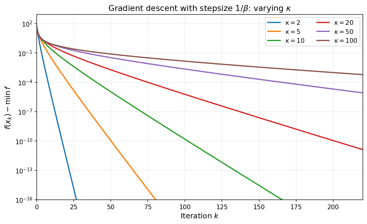
As a concrete numerical illustration, the plot below shows gradient descent with stepsize $\eta=1/\beta$ on convex quadratics with varying condition numbers, with all runs initialized at the origin. The vertical axis is $\log\bigl(f(x_k)-f^\ast\bigr)$ (shown on a semilog scale): larger $\kappa$ produces slower decay.
At this point we have extracted essentially the best guarantee available from one fixed stepsize by ensuring a contraction in every step, and then iterating the bound. The natural next question is whether coordinating multiple steps can outperform optimizing each step in isolation. The answer turns out to be yes, and leads to a dramatic improvement in iteration complexity wherein the linear dependence on $\kappa$ is replaced by a linear dependence on $\sqrt{\kappa}$.
3. Acceleration by Chebyshev Stepsizes
The analysis of gradient descent so far was quite crude in that it was based on lower-bounding the improvement in function value after $k$ iteration using a fixed step-size; in essence, the argument reduced to choosing a fixed step-size that guarantees the largest function value decrease in a single step and then iterating the bound. We now show that by monitoring performance across the entire time horizon, it is possible to choose a time-varying stepsize that yields a much faster rate of convergence. To see this, consider gradient descent with time-varying stepsizes $\eta_0, \eta_1, \ldots, \eta_{k-1}$. We saw that the error $e_j = x_j - x^\ast$ evolves as $e_{j+1} = (I - \eta_j A)\,e_j$. Therefore, after $k$ steps we have:
\[e_k = (I - \eta_{k-1}A)(I - \eta_{k-2}A)\cdots(I - \eta_0 A)\,e_0 = p_k(A)\,e_0,\]where $p_k$ is the degree-$k$ polynomial
\[p_k(\lambda) = \prod_{j=0}^{k-1}(1 - \eta_j \lambda).\]Note that we have $p_k(0) = 1$ regardless of the choice of stepsizes. Expanding $e_k$ in the eigenbasis of $A$ as before yields:
\[\begin{aligned} f(x_k) - f^\ast = \tfrac{1}{2}\|e_k\|_A^2 &= \tfrac{1}{2}\sum_{i=1}^d \lambda_i\, p_k(\lambda_i)^2\, c_i^2 \leq \max_{\lambda \in [\alpha, \beta]} p_k(\lambda)^2 \cdot \tfrac{1}{2}\|e_0\|_A^2. \end{aligned}\]Rearranging we deduce
\[\frac{f(x_k) - f^\ast}{f(x_0) - f^\ast} \leq \max_{\lambda \in [\alpha, \beta]} p_k(\lambda)^2.\]Fixed-stepsize gradient descent corresponds to the special case $p_k(\lambda) = (1 - \eta\lambda)^k$, but we are now free to choose any stepsizes. Notice that as we vary the stepsizes $\eta_0,\ldots,\eta_{k-1}$, any polynomial $p(\lambda)$ of degree at most $k$, having all real roots, and satisfying $p(0)=1$ can be realized as $p_k(\lambda)$. Thus choosing time-varying stepsizes is equivalent to choosing such a polynomial. The best possible convergence after $k$ steps is therefore determined by the minimax polynomial problem:
\[\min_{\substack{p \in \mathcal{P}^{r}_k \\ p(0) = 1}} \max_{\lambda \in [\alpha, \beta]} p(\lambda)^2. \tag{2}\]where $\mathcal{P}^r_k$ denotes the set of polynomials of degree at most $k$ with all real roots. The solution to this classical variational problem is described through so-called Chebyshev polynomials of the first kind.
Chebyshev polynomials
The Chebyshev polynomial of the first kind of degree $k$, denoted $T_k$, is defined recursively: set $T_0(x) = 1$ and $T_1(x) = x$ and define
\[T_{k+1}(x) = 2x\,T_k(x) - T_{k-1}(x) \qquad \forall k\geq 1.\]An equivalent characterization of Chebyshev polynomials is the expression
\[T_k(\cos\theta) = \cos(k\theta) \qquad \forall \theta \in [0,\pi].\]Chebyshev polynomials play a special role in numerical analysis because they solve the extremal problem:
Any degree-$k$ polynomial $p(x)$ with the same leading coefficient as $T_k$ satisfies
\[\max_{x\in [-1,1]} \lvert p(x)\rvert\geq \max_{x\in [-1,1]} \lvert T_k(x)\rvert=1.\]
In words, among all degree-$k$ polynomials with the same leading coefficient as $T_k$, the Chebyshev polynomial $T_k$ has the smallest maximum absolute value on $[-1,1]$. See the figure below that illustrates a few Chebyshev polynomial $T_k$.
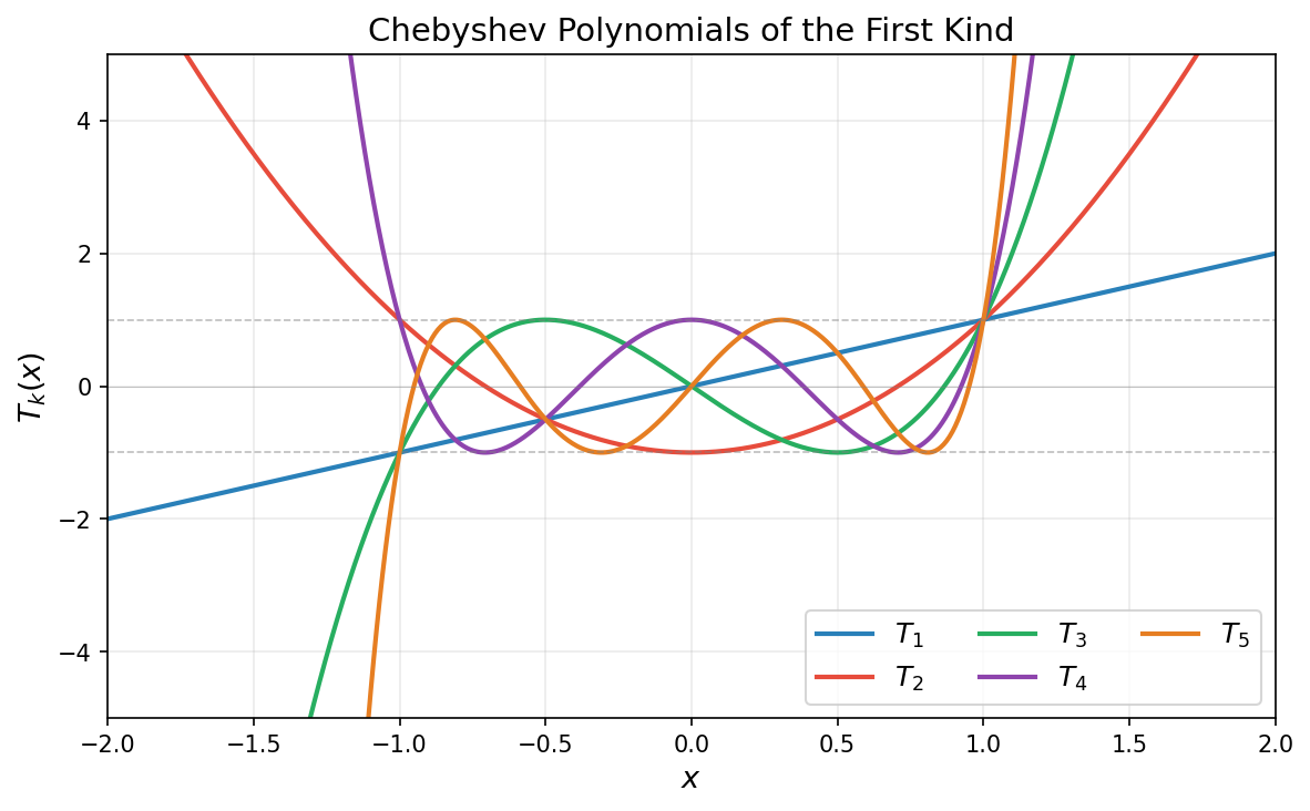
Chebyshev polynomials satisfy the following key properties:
-
Boundedness: The inequality $\lvert T_k(t)\rvert \leq 1$ holds for all $t \in [-1,1]$.
-
Roots: $T_k$ has $k$ roots in $(-1,1)$ at $t_j = \cos\left(\frac{(2j-1)\pi}{2k}\right)$ for $j = 1, \ldots, k$.
-
Explosion: For $t > 1$, we have $T_k(t) = \cosh(k\,\operatorname{arccosh}(t))$.
In summary, the Chebyshev polynomials $T_k$ are designed to be highly oscillatory on the interval $[-1,1]$ so as to stay bounded by one in absolute value, but this evidently forces these polynomials to grow rapidly outside the interval $[-1,1]$.
The optimal polynomial
Returning to gradient descent, let us see how Chebyshev polynomials yield a solution to the minimax problem $(2)$. We rescale the interval $[\alpha, \beta]$ to $[-1,1]$ with the affine change of coordinates $\varphi(\lambda)=\frac{\beta + \alpha - 2\lambda}{\beta - \alpha}$. Note that $\varphi$ sends $\lambda = 0$ to the point $\sigma := \frac{\beta + \alpha}{\beta - \alpha} = \frac{\kappa + 1}{\kappa - 1}$, assuming $\alpha>0$. Thus, under this substitution, any degree-$k$ polynomial $p(\lambda)$ with $p(0) = 1$ corresponds to a degree-$k$ polynomial $q=p\circ\varphi^{-1}$ with $q(\sigma) = 1$, and
\[\max_{\lambda \in [\alpha, \beta]}\lvert p(\lambda)\rvert = \max_{t \in [-1,1]}\lvert q(t)\rvert.\]We must therefore find the degree-$k$ polynomial $q$ with $q(\sigma) = 1$ that has the smallest maximum on $[-1,1]$. By properties 1 and 3 above, $T_k$ is bounded by $1$ on $[-1,1]$ while $T_k(\sigma) \gg 1$ for large $k$. This makes the rescaled polynomial
\[q_k^*(t):= \frac{T_k(t)}{T_k(\sigma)}\]an excellent candidate: it satisfies $q_k^{\ast}(\sigma) = 1$ and $\max_{t \in [-1,1]}\lvert q_k^{\ast}(t)\rvert = 1/T_k(\sigma)$, which is small because $T_k(\sigma)$ grows exponentially in $k$. Transforming back to the $\lambda$-variable, the optimal polynomial is
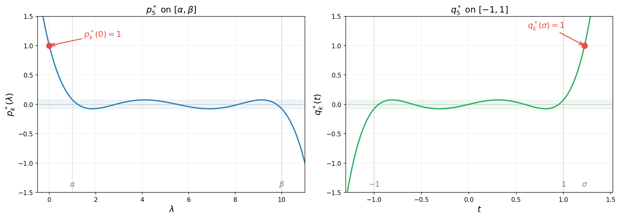
\[p_k^*(\lambda) :=(q_k^*\circ\varphi)(\lambda)= \frac{T_k\!\left(\frac{\beta + \alpha - 2\lambda}{\beta - \alpha}\right)}{T_k\!\left(\frac{\kappa + 1}{\kappa - 1}\right)}.\]Note that $p_k^*$ has all real roots. The figure below illustrates the reparametrization for $k=5$: on the left, $p_k^{\ast}$ satisfies the constraint $p_k^{\ast}(0)=1$ and oscillates with small amplitude on $[\alpha,\beta]$; on the right, $q_k^{\ast}$ satisfies $q_k^{\ast}(\sigma)=1$ and oscillates on $[-1,1]$ with the same small amplitude $1/T_k(\sigma)$.
The animation below shows $p_k^{\ast}(\lambda)$ on $[\alpha, \beta]$ for increasing degree $k$. As $k$ grows, the polynomial oscillates more rapidly yet its maximum amplitude $1/T_k(\sigma)$ shrinks exponentially—this is the mechanism behind the accelerated convergence.
Summarizing, we have the following lemma. Note that the first inequality holds as equality, as quickly follows from the extremal property of $T_k$. We omit the argument since it is not needed for what follows.
Lemma 3.1 (Chebyshev minimax). Suppose $\alpha>0$. Then with $\sigma = \frac{\kappa+1}{\kappa-1}$, the minimax value satisfies
\[\min_{\substack{p \in \mathcal{P}^r_k \\ p(0) = 1}} \max_{\lambda \in [\alpha,\beta]} \lvert p(\lambda)\rvert \leq \frac{1}{T_k(\sigma)} \leq 2\left(\frac{\sqrt{\kappa}-1}{\sqrt{\kappa}+1}\right)^k.\]Proof. We already proved the first inequality. For the second inequality, we use the identity $T_k(x) = \cosh(k\,\operatorname{arccosh}(x))$ valid for every real number $x>1$. Applying this identity with the quantity $\sigma$ gives the relation
\[\begin{aligned} \operatorname{arccosh}(\sigma) &= \ln\!\big(\sigma + \sqrt{\sigma^2 - 1}\big) = \ln\frac{\sqrt{\kappa}+1}{\sqrt{\kappa}-1}. \end{aligned}\]Consequently, the representation
\[\begin{aligned} T_k(\sigma) &= \cosh\!\left(k\ln\frac{\sqrt{\kappa}+1}{\sqrt{\kappa}-1}\right) = \frac{1}{2}\left[\left(\frac{\sqrt{\kappa}+1}{\sqrt{\kappa}-1}\right)^k + \left(\frac{\sqrt{\kappa}-1}{\sqrt{\kappa}+1}\right)^k\right] \geq \frac{1}{2}\left(\frac{\sqrt{\kappa}+1}{\sqrt{\kappa}-1}\right)^k, \end{aligned}\]holds. Taking reciprocals gives the second claim. This completes the proof. $\square$
Returning to choosing stepsizes for gradient descent, the roots of $p^{\ast}_k(\lambda)$ on $[\alpha, \beta]$ are the images of the Chebyshev roots $t_j$ under the inverse map $\varphi^{-1}(t) = \frac{\beta+\alpha}{2} - \frac{\beta-\alpha}{2}\,t$, yielding the stepsizes $\eta_j = 1/\lambda_j$. We thus have arrived at the main theorem of this section.
Theorem 3.1 (Chebyshev stepsizes). Define the stepsizes
\[\eta_j = \tfrac{1}{\lambda_j}~~ \textrm{where}~~\lambda_j = \tfrac{\beta + \alpha}{2} - \tfrac{\beta - \alpha}{2}\cos\!\left(\tfrac{(2j - 1)\pi}{2k}\right) ~~\textrm{for}~ j = 1, \ldots, k.\]Then as long as $\alpha>0$ the gradient descent iterates satisfy
\[f(x_k) - f^\ast \leq 4\left(\frac{\sqrt{\kappa} - 1}{\sqrt{\kappa} + 1}\right)^{2k}\bigl(f(x_0) - f^\ast\bigr). \tag{3}\]Proof. Combining the estimate $(2)$ and Lemma 3.1 directly yields \(\frac{f(x_k) - f^\ast}{f(x_0) - f^\ast} \leq \max_{\lambda \in [\alpha, \beta]} p_k^*(\lambda)^2 = \frac{1}{T_k(\sigma)^2}\leq 4\left(\frac{\sqrt{\kappa}-1}{\sqrt{\kappa}+1}\right)^{2k}.\) This completes the proof. $\square$
Thus, the iteration complexity of Chebyshev-accelerated gradient descent is $O(\sqrt{\kappa}\,\log((f(x_0)-f^\ast)/\varepsilon))$—a square-root improvement over the $O(\kappa\,\log((f(x_0)-f^\ast)/\varepsilon))$ complexity of fixed-stepsize gradient descent. For $\kappa = 100$, this is the difference between roughly $10$ and $100$ iterations.
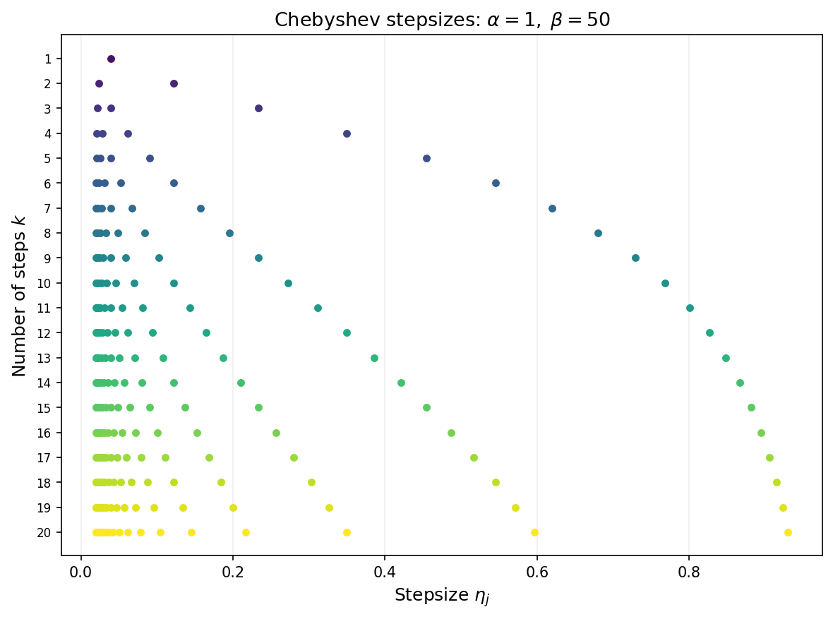
Visualizing the stepsizes and performance of the accelerated algorithm
Note that the convergence guarantees are not ``anytime’’. The stepsize must be determined with the number of total iterations $k$ in mind. The next figure shows the Chebyshev stepsizes for each choice of total iteration count $k$ from 1 to 20. Each row displays the $k$ stepsizes as points along the horizontal axis. As $k$ grows, the stepsizes fill out the interval $[1/\beta,\,1/\alpha]$ with increasing density near the endpoints—reflecting the characteristic clustering of Chebyshev roots.
The animation below overlays gradient descent (blue) and Chebyshev-accelerated GD (red) on the same ill-conditioned quadratic. The Chebyshev method reaches the minimizer much faster.
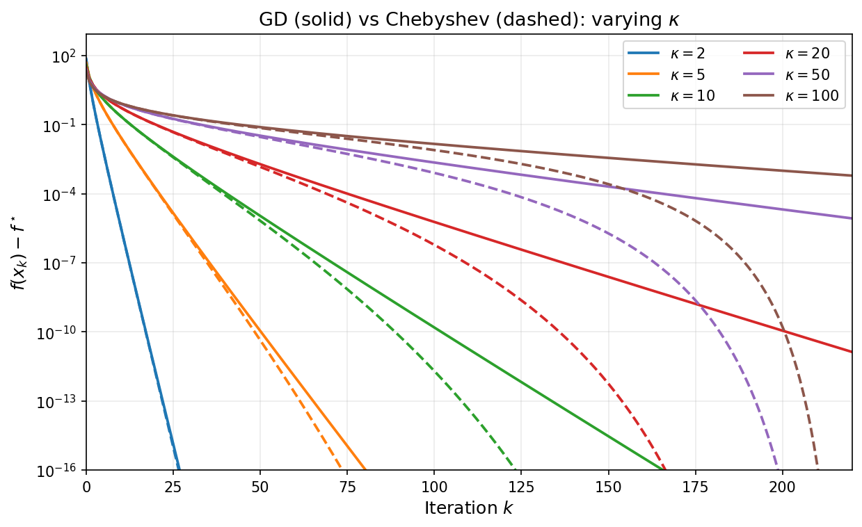
As a final illustration, the plot below overlays GD with stepsize $1/\beta$ (solid) and Chebyshev-accelerated GD with $k = 220$ (dashed) for varying condition numbers. The Chebyshev curves stay nearly flat during the cycle and then drop sharply near the final iteration, reaching machine precision much sooner than GD for every value of $\kappa$.
4. The Krylov Subspace Method and Conjugate Gradient
From polynomials to Krylov subspaces
The Chebyshev method discussed in Section 3 achieves the iteration complexity $O(\sqrt{\kappa}\,\ln((f(x_0)-f^\ast)/\varepsilon))$ by cleverly choosing time-varying stepsizes—but it requires advance knowledge of the extreme eigenvalues $\alpha$ and $\beta$. Moreover, the total number of iterations must be set in advance in order to define the stepsizes. A natural question arises:
Can we design an adaptive algorithm that matches this rate adaptively, without knowing the spectrum nor setting the time horizon?
The key observation is that gradient descent with any sequence of stepsizes produces iterates that lie in a specific linear subspace. Due to the recursion $x_{j+1} = x_j - \eta_j(Ax_j - b)$, one readily verifies the inclusion
\[x_k \in x_0 + \mathcal{K}_k(A, r_0),\]where $r_0 := b - Ax_0$ is the initial residual and
\[\mathcal{K}_k(A, r_0) := \mathrm{span}\{r_0,\, Ar_0,\, A^2 r_0,\, \ldots,\, A^{k-1}r_0\}\]is the Krylov subspace of order $k$. Both fixed-stepsize gradient descent and the Chebyshev method search within this subspace but do not fully exploit it. The natural idea is to search optimally within the Krylov subspace at each step.
The Krylov subspace method
The Krylov subspace method is the idealized algorithm that, at each step $k$, sets
\[x_k = \argmin_{x \,\in\, x_0 + \mathcal{K}_k(A,\,r_0)} f(x). \tag{4}\]It is illuminating to compare the exact performance of the Krylov method to that of gradient descent with time-varying stepsizes. Write as usual $e_0 = x_0 - x^\ast = \sum_{i=1}^d c_i v_i$ in the eigenbasis of $A$. Recall that optimizing over the stepsizes $\eta_0,\ldots,\eta_{k-1}$, yields the function-value guarantee for the last iterate of gradient descent:
\[f(x_k) - f^\ast \;=\;\min_{\substack{p \in \mathcal{P}^{r}_k \\ p(0) = 1}} \tfrac{1}{2}\sum_{i=1}^d \lambda_i\, c_i^2\, p(\lambda_i)^{2}. \tag{4a}\]For the Krylov method, any point $x \in x_0 + \mathcal{K}_k(A,r_0)$ can be written as $x = x_0 + q(A)\,r_0$ for some polynomial $q$ of degree at most $k-1$. Using the expression $r_0 = -A\,e_0$ this becomes
\[x - x^\ast \;=\; e_0 - q(A)\,A\,e_0 \;=\; p(A)\,e_0, \tag{5}\]where we define the polynomial $p(\lambda) = 1 - \lambda\,q(\lambda)$. As $q$ varies over polynomials of degree at most $k-1$, the polynomial $p$ varies over all of $\mathcal{P}_k$ with $p(0)=1$, with no real-root restriction. The defining property $(4)$ therefore yields the equality
\[f(x_k) - f^\ast \;=\; \min_{\substack{p \in \mathcal{P}_k \\ p(0) = 1}} \tfrac{1}{2}\sum_{i=1}^d \lambda_i\, c_i^2\, p(\lambda_i)^{2}\qquad \forall k. \tag{4b}\]The two expressions $(4a)$ and $(4b)$ differ in exactly one formal respect: the Krylov method optimizes over all polynomials with $p(0)=1$, whereas gradient descent is confined to those with real roots.
Theorem 4.1 (Krylov method convergence). Assuming $\alpha > 0$, the Krylov subspace method $(4)$ satisfies
\[f(x_k) - f^\ast \leq 4\left(\frac{\sqrt{\kappa} - 1}{\sqrt{\kappa} + 1}\right)^{2k}\bigl(f(x_0) - f^\ast\bigr) \qquad \forall k\geq 0.\]Moreover, the method converges in at most $m$ iterations, where $m$ is the number of distinct eigenvalues of $A$.
Proof. The linear rate follows directly from Theorem $3.1$: the $k$th iterate produced by the Chebyshev stepsizes lies in $x_0+\mathcal{K}_k(A,r_0)$, whereas the Krylov method minimizes $f$ over that entire affine space, and so cannot do worse.
To prove finite termination, observe that by $(4b)$ it suffices to exhibit a polynomial $p \in \mathcal{P}_m$ with $p(0)=1$ for which $\sum_{i=1}^d \lambda_i\,c_i^2\,p(\lambda_i)^2 = 0$, since this forces $f(x_m) = f^\ast$ and hence $x_m = x^\ast$. Take
\[p(\lambda):=\prod_{i=1}^m\left(1-\frac{\lambda}{\lambda_i}\right),\]where $\lambda_1,\ldots,\lambda_m$ are the distinct eigenvalues of $A$. Then $p$ has degree $m$, satisfies $p(0)=1$, and vanishes at every eigenvalue of $A$, so the sum is zero as required. $\square$
The convergence bound in Theorem 4.1 is identical to the Chebyshev bound in Theorem 3.1, and the iteration complexity has the same order $O(\sqrt{\kappa}\,\ln((f(x_0)-f^\ast)/\varepsilon))$. Importantly, the Krylov method achieves this complexity without knowing $\alpha$ or $\beta$ and without requiring to specify the time horizon $k$; moreover, finite termination provides an absolute guarantee of at most $m$ steps, where $m$ is the number of distinct eigenvalues. In practice, clustered eigenvalues lead to far fewer iterations than the worst-case bound suggests.
The Conjugate Gradient algorithm implements the Krylov method
The Krylov subspace method $(4)$ is conceptual: a direct implementation would solve a $k$-dimensional linear optimization problem at each step, with cost growing as $k$ increases. The Conjugate Gradient (CG) algorithm is an implementation of the Krylov method that uses only one matrix-vector product per iteration.
The key idea is to iteratively build a basis of the Krylov subspaces that is orthogonal with respect to the inner product $\langle x,y\rangle_A=x^\top Ay$, so that each successive minimization reduces to a single line search. Conceptually, this basis is formed by a Gram–Schmidt process. The special structure of Krylov subspaces ensures that each Gram–Schmidt update requires only the immediately preceding direction—a short recurrence—rather than all previous directions.
Concretely, suppose that we have constructed an $A$-orthogonal basis $\lbrace p_i\rbrace _{i=0}^{k-1}$ for $\mathcal{K}_{k}$ and that we have available a minimizer $x_k$ of $f$ on $x_0 + \mathcal{K}_k$. Let us see how we can efficiently extend the $A$-orthogonal basis to $\mathcal{K}_{k}$ and construct the minimizer $x_{k+1}$ of $f$ on $x_0 + \mathcal{K}_{k+1}$. To this end, define the residuals $$r_i=-\nabla f(x_i)=b-Ax_i.$$
Observe that we may write $r_k=b-Ax_k=r_0-A(x_k-x_0)$ and therefore $r_k$ lies in $\mathcal{K}_{k+1}$. Now, set $$p_{k}=r_k+\beta_{k-1} p_{k-1},$$ for a constant $\beta_{k-1}$ to be chosen. We would like to ensure that $p_{k}$ is $A$-orthogonal to $\lbrace p_i\rbrace _{i=0}^{k-1}$ . To this end, setting $p_{k}^\top Ap_{k-1}=0$ yields the unique choice of $\beta_{k-1}=-\frac{r_k^\top Ap_{k-1}}{p_{k-1}^\top Ap_{k-1}}$. Now for any $i<k-1$ we compute $$p_{k}^{\top}A p_{i}=r_k^\top A p_{i}+\beta_{k-1}p_{k-1}^{\top}Ap_i.$$ Observe that $p_{k-1}^{\top}Ap_i=0$ by assumed A-orthogonality of $\lbrace p_i\rbrace _{i=0}^{k-1}$ and $r_k^\top A p_{i}=0$ because $A p_{i}$ lies in $\mathcal{K}_{i+1}$ and the optimality conditions for $x_k$ imply $r_k\perp K_{k}$. Thus $\lbrace p_i\rbrace _{i=0}^{k}$ is indeed an A-orthogonal basis for $\mathcal{K}_{k}$. It remains to declare $$x_{k+1}=\argmin_{\eta} f(x_k+\eta p_{k}). \tag{6}$$Indeed, taking the derivative in $\eta$ implies $r_{k+1}\perp p_{k}$ and for any $i<k$ we have orthogonality $$r_{k+1}^\top p_{i}=(r_k-\eta_k Ap_k)^{\top}p_i=r_k^\top p_i-\eta_k p_k^\top Ap_i=0,$$ where $\eta_k$ is the minimizer of $(6)$. Thus $x_{k+1}$ is indeed the minimizer of $f$ on $x_0+\mathcal{K}_{k+1}$. The algorithm we just constructed is called the conjugate gradient method and is summarized in the following.
Algorithm 1 (Conjugate Gradient Method)
Input: $x_0 \in \mathbb{R}^d$
- Set $r_0 = b - Ax_0$, $\;p_0 = r_0$
- For $k = 0, 1, 2, \ldots$ do:
- $\qquad \eta_k = \dfrac{r_k^\top r_k}{p_k^\top A p_k}$
- $\qquad x_{k+1} = x_k + \eta_k\, p_k$
- $\qquad r_{k+1} = r_k - \eta_k\, A p_k$
- $\qquad \beta_k = -\dfrac{r_{k+1}^\top A p_k}{p_k^\top A p_k}$
- $\qquad p_{k+1} = r_{k+1} + \beta_k\, p_k$
Each iteration of the conjugate gradient method requires one matrix-vector product $Ap_k$, the same per-step cost as gradient descent. The vectors $r_k = b - Ax_k$ are the residuals satisfying $r_k = -\nabla f(x_k)$, while the vectors $p_k$ are the search directions. The stepsize $\eta_k$ minimizes $f$ along the ray $x_k + \eta\, p_k$, while $\beta_k$ ensures $A$-orthogonality of consecutive search directions.
Remark. In the literature, the update for $\beta_k$ is usually written in the equivalent form $\beta_k = \lVert r_{k+1}\rVert ^2/\lVert r_k\rVert ^2$. The equivalence is straightforward to establish from the residual recursion $Ap_k = (r_k - r_{k+1})/\eta_k$; we omit the argument for brevity.
Visualizing CG
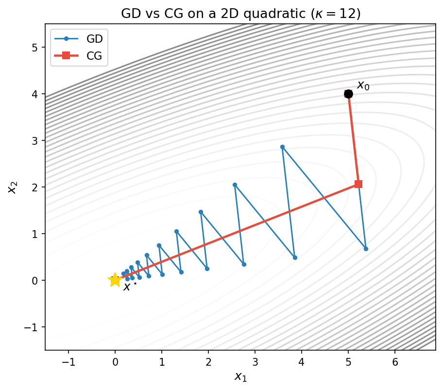
The figure below compares GD and CG on the same ill-conditioned 2D quadratic ($\kappa = 12$). Gradient descent (blue) zig-zags along the narrow valley, requiring many iterations to approach the minimum. CG (red) reaches the minimum in exactly 2 steps—the dimension of the problem—by choosing $A$-orthogonal search directions that span the full space.
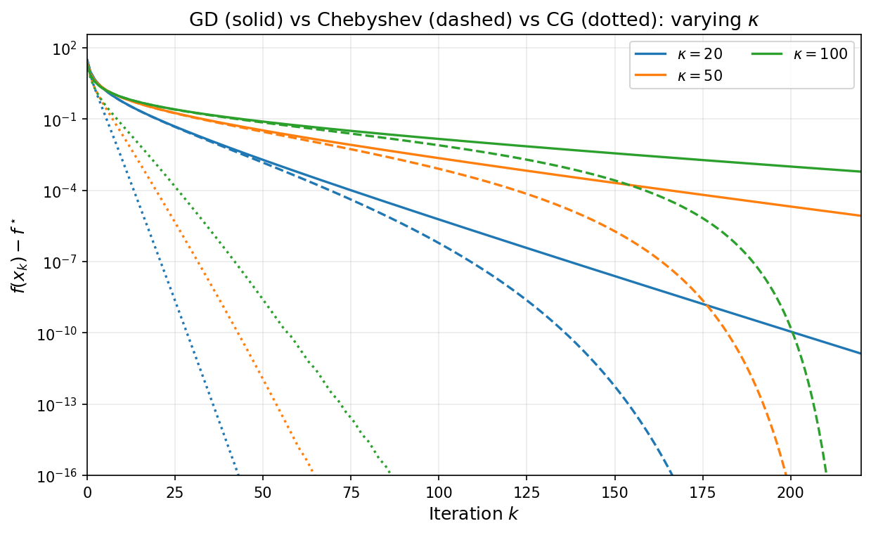
The next figure repeats the varying-$\kappa$ experiment from Section 3, now with CG (dotted) added alongside GD (solid) and Chebyshev (dashed). For each condition number, CG converges much faster than gradient descent and the Chebyshev method—without requiring knowledge of $\alpha$ or $\beta$, and without presetting the number of iterations.
6. Sublinear Rates in the Positive Semidefinite Case
Motivation
The convergence guarantees of the previous sections all rely on the assumption $\alpha > 0$—that is, $A$ is positive definite. When $\alpha$ is very close to zero, however, the condition number $\kappa = \beta/\alpha$ can become arbitrarily large and the linear convergence bounds of Theorems 1, 2, and 3 essentially become vacuous. This situation arises often in practice. As a concrete example let us look at the prototypical problem of solving a linear system generated by a kernel matrix.
Example (Kernel matrices and spectral decay). A kernel function $k\colon\mathbb{R}^d\times\mathbb{R}^d\to\mathbb{R}$ is a symmetric function such that the kernel matrix $K\in\mathbb{R}^{n\times n}$ defined by $K_{ij}=k(x_i,x_j)$ is positive semidefinite for every finite collection of points $x_1,\dots,x_n\in\mathbb{R}^d$. Kernel matrices are ubiquitous: they arise in Gaussian process regression, support vector machines, kernel ridge regression, and radial-basis-function interpolation. Given a target vector $y\in\mathbb{R}^n$, the core computational task reduces to solving the linear system
\[K\alpha = y,\]which is exactly the quadratic minimization problem $\min_\alpha \tfrac{1}{2}\alpha^\top K\alpha - y^\top \alpha$.
Two of the most widely used kernels depend only on the $\ell_2$ distance $\lVert x-y\rVert $ and a length-scale parameter $\sigma>0$, called the bandwidth. The Gaussian (RBF) kernel is
\[k_{\mathrm{RBF}}(x,y)=\exp\!\left(-\frac{\|x-y\|^2}{2\sigma^2}\right).\]It is infinitely differentiable ($C^\infty$). The Laplace kernel is \(k_{\mathrm{Lap}}(x,y)=\exp\!\left(-\frac{\|x-y\|}{\sigma}\right).\) It is continuous but not differentiable at the origin ($C^0$). The Laplace kernel is the Matérn kernel with $m=\tfrac12$. More generally, the Matérn family interpolates between Laplace and Gaussian by introducing a smoothness parameter $m>0$. The general Matérn kernel is
\[k_m(x,y)=\frac{2^{1-m}}{\Gamma(m)}\left(\frac{\sqrt{2m}\,\|x-y\|}{\sigma}\right)^m K_m\!\left(\frac{\sqrt{2m}\,\|x-y\|}{\sigma}\right),\]where $K_m$ is the modified Bessel function of the second kind. The parameter $m$ controls the smoothness: the Matérn kernel with parameter $m$ is $\lceil m\rceil -1$ times continuously differentiable. Several important finite-$m$ cases, together with the Gaussian limit, are summarized in the following table:
| Kernel | $m$ | Closed form | Smoothness |
|---|---|---|---|
| Laplace | $\tfrac12$ | $\exp\bigl(-\tfrac{\lVert x-y\rVert }{\sigma}\bigr)$ | $C^0$ |
| Matérn 3/2 | $\tfrac32$ | $\bigl(1+\tfrac{\sqrt{3}\lVert x-y\rVert }{\sigma}\bigr)\exp\bigl(-\tfrac{\sqrt{3}\lVert x-y\rVert }{\sigma}\bigr)$ | $C^1$ |
| Matérn 5/2 | $\tfrac52$ | $\bigl(1+\tfrac{\sqrt{5}\lVert x-y\rVert }{\sigma}+\tfrac{5\lVert x-y\rVert ^2}{3\sigma^2}\bigr)\exp\bigl(-\tfrac{\sqrt{5}\lVert x-y\rVert }{\sigma}\bigr)$ | $C^2$ |
| Gaussian (RBF) | $\infty$ | $\exp\bigl(-\tfrac{\lVert x-y\rVert ^2}{2\sigma^2}\bigr)$ | $C^\infty$ |
In the limit $m\to\infty$ the Matérn kernel recovers the Gaussian kernel.
For reasonable distributions of data points (e.g., Gaussian, uniform, or with a bounded density on a compact set), the eigenvalues of the normalized kernel matrix $(1/n)K$ resemble those of an associated linear integral operator, whose spectral decay can be analyzed explicitly. More precisely suppose that the points $x_1,\ldots, x_n$ are drawn iid from a distribution $\nu$ on $\mathbb{R}^d$. For any function $f\in L_2(\nu)$ define the $n$-dimensional vector
\[f^{(n)}=\tfrac{1}{\sqrt{n}}(f(x_1),\ldots, f(x_n)).\]Then we may write the quadratic form of $\frac{1}{n}K$ as
\[(f^{(n)})^\top (\tfrac{1}{n}K)(f^{(n)})=\frac{1}{n^2}\sum_{i,j}k(x_i,x_j)f(x_i)f(x_j)=\int\int k(x,x')f(x)f(x')~dP_n(x)dP_n(x'),\]where $dP_n=\frac{1}{n}\sum_{i=1}^n\delta_{x_i}$ is the atomic measure on the samples. As $n$ tends to infinity, under mild assumptions, the right-hand-side tends to the integral quadratic form $T\colon L_2(\nu)\times L_2(\nu)\to \mathbb{R}$ given by
\[T(f,f)=\int\int k(x,x')f(x)f(x')~d\nu(x)d\nu(x').\]Note that this quadratic form is generated by the linear operator on functions $T\colon L_2(\nu)\to L_2(\nu)$ given by
\[(Tf)(x)=\int k(x,x')f(x')\,d\nu(x').\]Heuristically, in the large-sample limit the eigenvalues of $\tfrac{1}{n}K$ approximate those of the integral operator $T$. Let $\mu_1\geq\mu_2\geq\cdots$ denote the eigenvalues of $T$, and let $p$ denote the intrinsic dimension of the data support. The end result is the following asymptotic estimate that holds for all sufficiently large eigenvalue indices $i$:
| Kernel | Eigenvalue decay | Rate for $\mu_i$ |
|---|---|---|
| Laplace ($m=\tfrac12$) | polynomial | $\mu_i\asymp i^{-(1+p)/p}$ |
| Matérn (smoothness $m$) | polynomial | $\mu_i\asymp i^{-(2m+p)/p}$ |
| Gaussian (RBF) | super-exponential | $\mu_i\lesssim C\exp(-c\, i^{2/p})$ |
As a consequence, kernel matrices are typically extremely ill-conditioned: the effective condition number $\lambda_1/\lambda_n$ grows rapidly with $n$, and for large $n$ many eigenvalues are numerically zero. This is precisely the regime where the positive definite theory becomes vacuous.
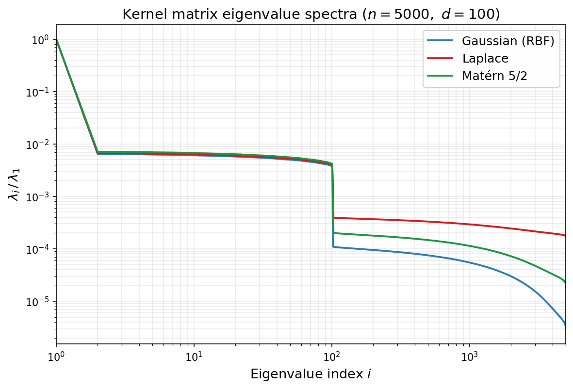
The figure below illustrates this phenomenon on synthetic data. We draw $n=5000$ points independently from the standard Gaussian distribution $\mathcal{N}(0,I_{100})$ in $\mathbb{R}^{100}$, use the same sample for all three kernels, choose the bandwidth $\sigma$ by the median heuristic, and plot the normalized eigenvalues $\lambda_i/\lambda_1$ on a log-log scale. A noticeable bend appears around index $i\approx d=100$; this is a finite-sample crossover caused by the interaction between the ambient dimension, the sampling distribution, and the kernel bandwidth, rather than a direct prediction of the asymptotic estimates above. The asymptotic theory instead describes the tail behavior after such pre-asymptotic effects: past the bend, the three kernels separate clearly. The Gaussian kernel (blue) exhibits the fastest decay, the Laplace kernel (red) the slowest, and the Matérn 5/2 kernel (green) is intermediate, in qualitative agreement with the rates in the table.
We will now develop convergence guarantees for all of the methods we have seen—gradient descent, Chebyshev-accelerated gradient descent, and the Krylov method—that are insensitive to the minimal eigenvalue of $A$. The price to pay is that the logarithmic dependence on $1/\varepsilon$ in the positive definite case degrades to a polynomial dependence on $1/\varepsilon$.
Setup
We consider the same quadratic objective $f(x) = \tfrac{1}{2}x^\top Ax - b^\top x$, but now we allow $\alpha = 0$. We assume throughout that $b \in \mathrm{range}(A)$, ensuring that the solution set
\[S = \{x \in \mathbb{R}^d : Ax = b\}\]is nonempty and we let $x^{\ast}\in S$ be arbitrary.
The eigenvalues of $A$ are ordered as
\[0 = \lambda_1 = \cdots = \lambda_r < \lambda_{r+1} \leq \cdots \leq \lambda_d = \beta,\]where $r \geq 1$ is the dimension of $\ker(A)$.
Gradient descent
We begin with the convergence rate of gradient descent. The key idea is that we have previously shown the exact relation \(f(x_k) - f^\ast = \frac{1}{2}\sum_{i=1}^{d}\lambda_i(1-\eta\lambda_i)^{2k}\,c_i^2\) where $\eta$ is the stepsize and $c_i$ are the coefficients of the initial error in the eigenbasis of $A$. Previously, we pulled out $\sup_{\lambda\in [\alpha,\beta]}(1-\eta\lambda)^{2k}$ from the sum. We now instead pull out $\sup_{\lambda\in [\alpha,\beta]}\lambda(1-\eta\lambda)^{2k}$.
Theorem 6.1 (Sublinear convergence of gradient descent). With stepsize $\eta = 1/\beta$, the gradient descent iterates satisfy
\[f(x_k) - f^\ast \leq \frac{\beta}{2(2k+1)}\,\|x_0 - x^\ast\|^2 \tag{7}.\]Proof. Writing out the initial error $e_0=x_0-x^\ast=\sum_{i=1}^d c_i v_i$ in the eigen-basis of $A$ yields
\[f(x_k) - f^\ast = \frac{1}{2}\sum_{i=1}^{d}\lambda_i(1-\lambda_i/\beta)^{2k}\,c_i^2 \leq \frac{1}{2}\max_{\lambda \in [0,\beta]}\lambda(1-\lambda/\beta)^{2k}\cdot\|e_0\|^2.\]Elementary calculus shows $\sup_{t\in [0,1]}t(1-t)^{q}=\frac{1}{1+q}(\frac{q}{1+q})^q\leq \frac{1}{1+q}$. Therefore setting $q=2k$ yields
\[\max_{\lambda \in (0,\beta]}\lambda(1-\lambda/\beta)^{2k} \leq \frac{\beta}{2k+1},\]which completes the proof. $\square$
From Theorem 6.1, converting to complexity, the bound $f(x_k) - f^\ast \leq \varepsilon$ is guaranteed to hold whenever
\[k \geq \frac{\beta\,\|x_0 - x^\ast\|^2}{4\varepsilon}.\]Thus the iteration complexity is
\[O\!\left(\frac{\beta\,\|x_0 - x^\ast\|^2}{\varepsilon}\right).\]Compared with the $O(\kappa\,\ln(1/\varepsilon))$ complexity of gradient descent in the positive definite case, the dependence on accuracy has changed from logarithmic to polynomial: achieving an additional digit of accuracy now requires a tenfold increase in iterations, rather than a fixed additive cost. This is the hallmark of sublinear convergence.
Note that an important feature of Theorem 6.1 is that the convergence bound involves the squared Euclidean distance $\lVert x_0 - x^\ast\rVert ^2$ rather than the initial function gap $f(x_0) - f^\ast$, and this is unavoidable.
Acceleration by Chebyshev stepsizes
As in the positive definite case, the $O(1/k)$ rate of fixed-stepsize gradient descent can be improved by varying the stepsize across iterations. Recall that the Chebyshev stepsizes arose in the positive definite case from the fact that the Chebyshev polynomial of the first kind $T_k$ minimizes $\max_{\lambda \in [-1,1]} p(\lambda)^2$ over all degree at most $k$ polynomials with the same leading coefficient. In the positive semidefinite case, the Chebyshev polynomials of the second kind will play an analogous role.
Chebyshev polynomials of the second kind
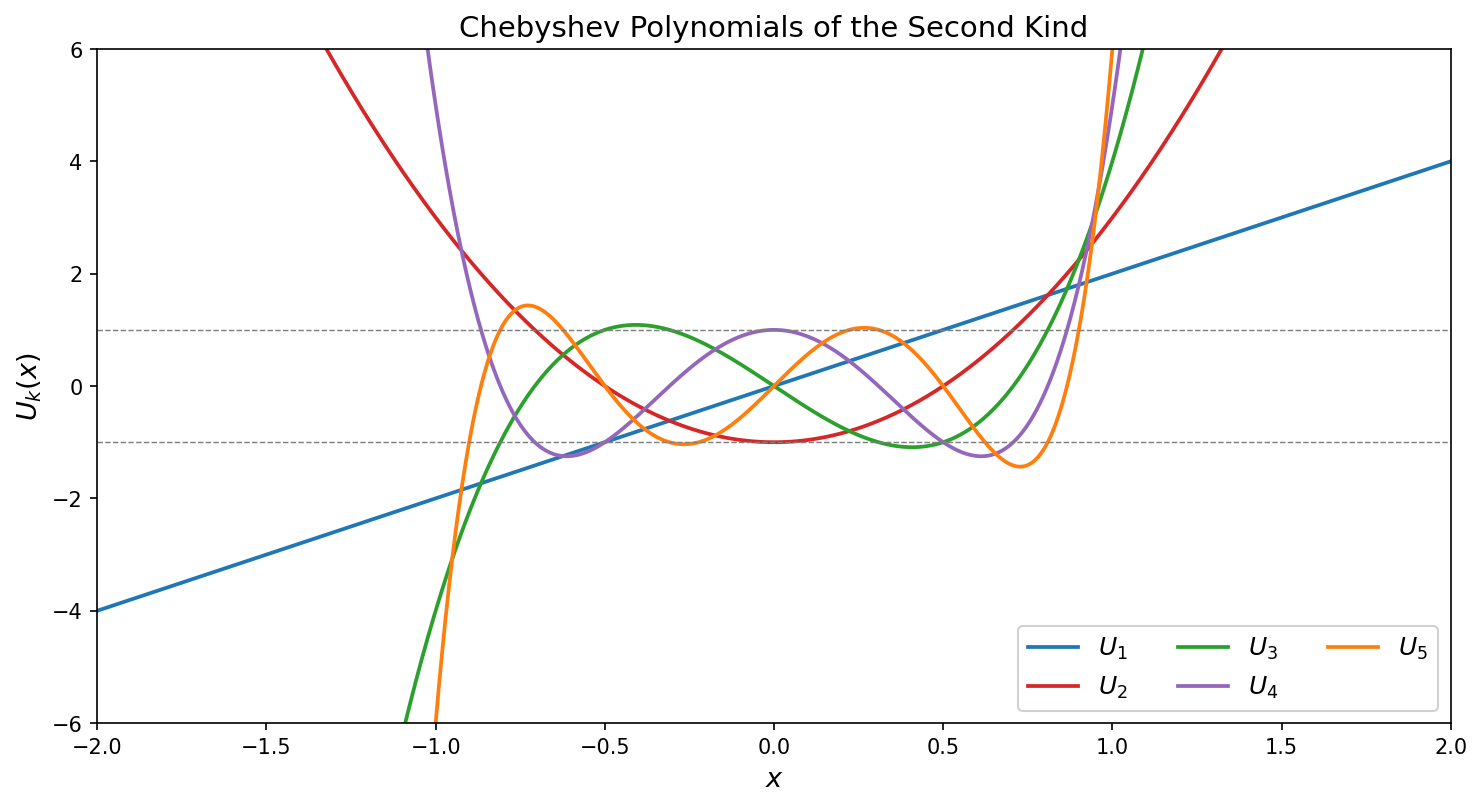
Chebyshev polynomials of the second kind are defined by the same recurrence as $T_k$ but with a different initial condition: set $U_0(x) = 1$ and $U_1(x) = 2x$ and define
\[U_{j+1}(x) = 2x\,U_j(x) - U_{j-1}(x) \qquad \forall j\geq 1.\]An equivalent trigonometric characterization is
\[U_j(\cos\theta) = \frac{\sin\bigl((j+1)\theta\bigr)}{\sin\theta},\]from which one directly sees $U_j(1) = j+1$. See the figure below.
The Chebyshev polynomials of the second kind solve a weighted analogue of the extremal problem for $T_k$:
Any degree-$k$ polynomial $p(x)$ with the same leading coefficient as $U_k$ satisfies
\[\max_{x\in [-1,1]} \sqrt{1-x^2}\,\lvert p(x)\rvert\geq \max_{x\in [-1,1]} \sqrt{1-x^2}\,\lvert U_k(x)\rvert=1.\]
The equality on the right follows from the identity $\sqrt{1-x^2}\,U_k(x) = \sin((k+1)\theta)$ when $x=\cos\theta$. As we will see, the weight $\sqrt{1-x^2}$ is precisely what arises from the extra factor of $\lambda$ in the PSD minimax problem after the change of variables.
The key properties, paralleling those of $T_k$, are:
- Boundedness: $\lvert U_k(\cos\theta)\rvert \leq k+1$ for all $\theta$, and moreover $\lvert \sin\theta\, U_k(\cos\theta)\rvert = \lvert\sin((k+1)\theta)\rvert \leq 1$.
- Roots: $U_{k}$ has $k$ roots in $(-1,1)$ at $\cos(j\pi/(k+1))$ for $j = 1, \ldots, k$.
- Growth at edges: $U_k(1) = k+1$, so $U_k$ grows polynomially at $x=1$, in contrast to the exponential growth of $T_k$.
We now linearly reparametrize and rescale the $U_{k-1}$ and define \(\phi_k(\lambda) = \left(1 - \frac{\lambda}{\beta}\right)\frac{U_{k-1}(1 - 2\lambda/\beta)}{k}.\) Note that we have $\phi_k(0) = 1$ and the roots of $\phi_k$ on $[0,\beta]$ are $\lambda_j = \beta\sin^2(j\pi/(2k))$ for $j = 1, \ldots, k$.
Lemma 6.2 (Chebyshev minimax, PSD case). The polynomial $\phi_k$ satisfies
\[\max_{\lambda \in [0,\beta]}\,\lambda\,\phi_k(\lambda)^2 \leq \frac{\beta}{4k^2}. \tag{10}\]Proof. Substitute $\cos\theta = 1 - 2\lambda/\beta$ for $\theta \in [0,\pi]$, so that $\lambda = \beta\sin^2(\theta/2)$ and $1 - \lambda/\beta = \cos^2(\theta/2)$. The Chebyshev identity gives $U_{k-1}(\cos\theta) = \sin(k\theta)/\sin\theta$, and the factorization $\sin\theta = 2\sin(\theta/2)\cos(\theta/2)$ yields
\[\begin{aligned} \lambda\,\phi_k(\lambda)^2 &= \beta\sin^2(\theta/2)\cdot\cos^4(\theta/2)\cdot\frac{\sin^2(k\theta)}{k^2\sin^2\theta} \\[4pt] &= \beta\sin^2(\theta/2)\cdot\cos^4(\theta/2)\cdot\frac{\sin^2(k\theta)}{4k^2\sin^2(\theta/2)\cos^2(\theta/2)} \\[4pt] &= \frac{\beta\cos^2(\theta/2)\,\sin^2(k\theta)}{4k^2}. \end{aligned}\]Since $\cos^2(\theta/2) \leq 1$ and $\sin^2(k\theta) \leq 1$ for all $\theta$, the claim follows. $\square$
We are now ready to see the accelerated rate.
Theorem 6.2 (Chebyshev stepsizes, PSD case). Define the stepsizes
\[\eta_j = \frac{1}{\beta\sin^2(j\pi/(2k))} \qquad \textrm{for}~ j = 1, \ldots, k.\]Then the gradient descent iterates satisfy
\[f(x_k) - f^\ast \leq \frac{\beta}{8k^2}\,\|x_0 - x^\ast\|^2. \tag{9}\]Proof. Write the initial error in the eigenbasis of $A$ as $ e_0=x_0-x^\ast=\sum_{i=1}^d c_i v_i. $ For gradient descent with stepsizes $\eta_1,\dots,\eta_k$, define the degree-$k$ polynomial $ p_k(\lambda):=\prod_{j=1}^k(1-\eta_j\lambda). $ By the choice $ \eta_j = \frac{1}{\beta\sin^2(j\pi/(2k))} $ we have $ p_k(\lambda)=\phi_k(\lambda). $ Therefore, the general error formula from Section 2 gives \(f(x_k) - f^\ast = \tfrac{1}{2}\sum_{i=1}^d \lambda_i\, \phi_k(\lambda_i)^2\, c_i^2 \leq \tfrac{1}{2}\max_{\lambda \in [0,\beta]} \lambda\,\phi_k(\lambda)^2 \sum_{i=1}^d c_i^2.\) Applying Lemma 6.2 and using $\sum_{i=1}^d c_i^2=\lVert e_0\rVert ^2=\lVert x_0-x^\ast\rVert ^2$, we obtain \(f(x_k) - f^\ast \leq \tfrac{1}{2}\cdot\frac{\beta}{4k^2}\cdot\|x_0-x^\ast\|^2 = \frac{\beta}{8k^2}\,\|x_0 - x^\ast\|^2.\) This completes the proof. $\square$
Thus, the iteration complexity of the Chebyshev accelerated algorithm is $O(\sqrt{\beta\,\lVert x_0 - x^\ast\rVert ^2/\varepsilon})$—a square-root improvement over the $O(\beta\,\lVert x_0 - x^\ast\rVert ^2/\varepsilon)$ complexity of fixed-stepsize gradient descent. This is a quadratic improvement in the complexity.
The corresponding stepsize schedule in the positive semidefinite case is shown below for several values of $k$.
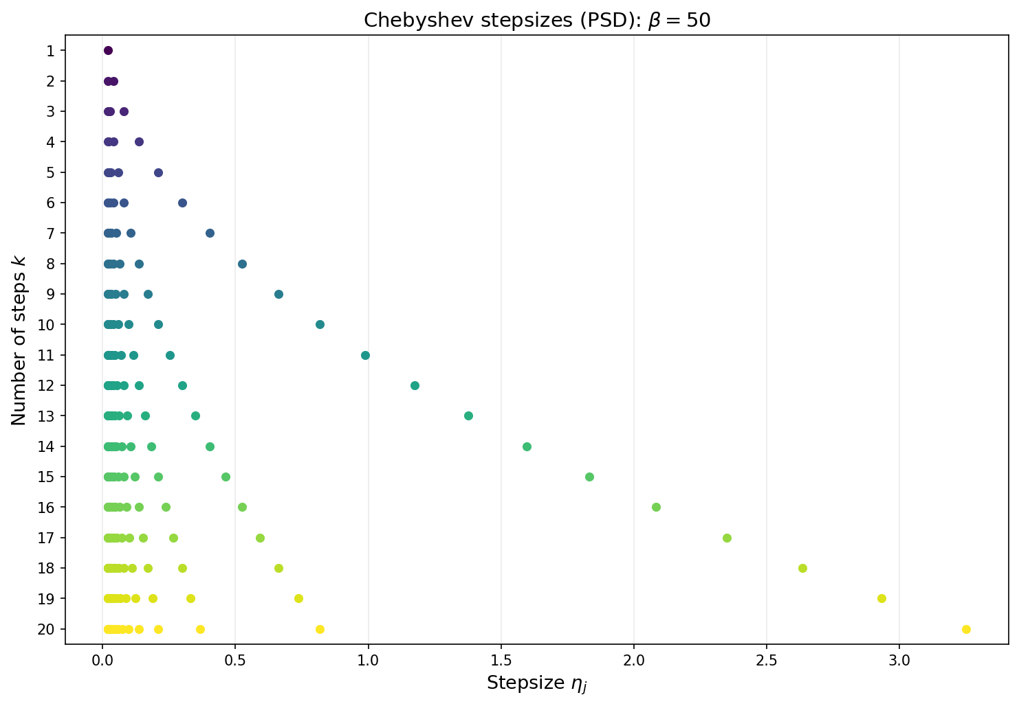
As in the positive definite case, the Chebyshev stepsizes require knowledge of $\beta$ and the total number of iterations $k$ must be fixed in advance.
Conjugate gradient in the positive semidefinite case
The Krylov subspace method in the PSD setting is defined exactly as before: at step $k$, it minimizes $f$ over the affine space \(x_0+\mathcal{K}_k(A,r_0).\) The only new issue is that $A$ may be singular. However, since $b\in\mathrm{range}(A)$ and $Ax_0\in\mathrm{range}(A)$, the residual $ r_0=b-Ax_0 $ lies in $\mathrm{range}(A)$. Therefore the entire Krylov subspace $\mathcal{K}_k(A,r_0)$ is contained in $\mathrm{range}(A)$, and $A$ is positive definite on that subspace. Consequently, the same short-recurrence argument from Section 4 shows that, until termination, the conjugate gradient method is well-defined and implements the PSD Krylov method: at each step, the CG iterate $x_k$ minimizes $f$ over $x_0+\mathcal{K}_k(A,r_0)$. With this observation in hand, the convergence analysis is immediate from Theorem 6.2, exactly as in the positive definite case.
Theorem 6.3 (CG convergence, PSD case). The CG iterates satisfy
\[f(x_k) - f^\ast \leq \frac{\beta}{8k^2}\,\|x_0 - x^\ast\|^2, \tag{11}\]and CG terminates in at most $m$ iterations, where $m$ is the number of distinct nonzero eigenvalues of $A$.
Proof. The rate follows directly from Theorem 6.2: the $k$th iterate produced by the PSD Chebyshev stepsizes lies in $x_0+\mathcal{K}_k(A,r_0)$, whereas CG minimizes $f$ over that entire affine space and so cannot do worse. $\square$
The bound $(11)$ matches the PSD Chebyshev bound $(9)$; the gain of CG is that it attains this behavior adaptively, without requiring $\beta$ or a preset horizon.
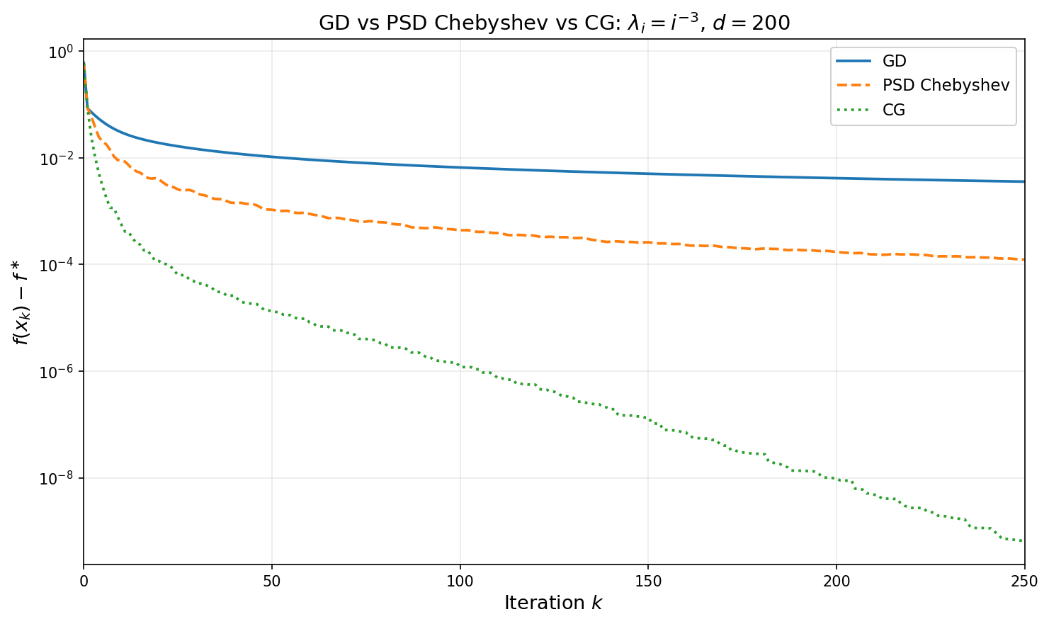
Numerical illustration
The figure below compares GD, PSD Chebyshev, and CG on a $d=200$ dimensional quadratic whose spectrum follows the power law $\lambda_i = i^{-3}$ (condition number $\approx 8\times 10^6$). For each horizon $k$, the PSD Chebyshev point plotted is the iterate after running all $k$ stepsizes from $x_0$. The sublinear separation between GD ($O(1/k)$) and Chebyshev ($O(1/k^2)$) is clearly visible, while CG reaches high accuracy in far fewer iterations.
Related Literature
The results discussed in these notes are largely classical in numerical optimization, Krylov methods, inverse problems, and random matrix theory. The novelty of these notes is mostly synthesis and alignment of viewpoints: optimization complexity bounds, Krylov polynomial optimality, source-condition regularity, and random-matrix spectral asymptotics are presented in one unified quadratic framework.
- Gradient descent and first-order complexity. Linear-rate GD analysis for strongly convex quadratics and condition-number dependence are standard; see [Pol64, Nes04, Nes18].
- Chebyshev acceleration and semi-iterative methods. The minimax polynomial viewpoint and Chebyshev stepsizes are classical; see [Var62, You71, Saa03].
- Conjugate gradient and Krylov optimality. Foundational CG/Krylov results originate in [HS52, Lan52]; modern treatments include [Saa03, Gre97].
References
- [HS52] Hestenes, M. R., and Stiefel, E. (1952). Methods of conjugate gradients for solving linear systems. Journal of Research of the National Bureau of Standards.
- [Lan52] Lanczos, C. (1952). An iteration method for the solution of the eigenvalue problem of linear differential and integral operators. Journal of Research of the National Bureau of Standards.
- [Pol64] Polyak, B. T. (1964). Some methods of speeding up the convergence of iteration methods. USSR Computational Mathematics and Mathematical Physics.
- [Var62] Varga, R. S. (1962). Matrix Iterative Analysis. Prentice-Hall.
- [You71] Young, D. M. (1971). Iterative Solution of Large Linear Systems. Academic Press.
- [Saa03] Saad, Y. (2003). Iterative Methods for Sparse Linear Systems (2nd ed.). SIAM.
- [Gre97] Greenbaum, A. (1997). Iterative Methods for Solving Linear Systems. SIAM.
- [Nes04] Nesterov, Y. (2004). Introductory Lectures on Convex Optimization. Kluwer.
- [Nes18] Nesterov, Y. (2018). Lectures on Convex Optimization (2nd ed.). Springer.
Summary
Worst-case iteration complexity.
| Method | Positive definite ($\alpha > 0$) | Positive semidefinite ($\alpha = 0$) |
|---|---|---|
| Gradient descent | $O(\kappa\,\ln(1/\varepsilon))$ | $O(\beta\,\lVert x_0 - x^\ast\rVert ^2/\varepsilon)$ |
| Chebyshev GD / Conjugate Gradient | $O(\sqrt{\kappa}\,\ln(1/\varepsilon))$ (CG: at most $m\le d$ steps) | $O(\sqrt{\beta\,\lVert x_0 - x^\ast\rVert ^2/\varepsilon})$ (CG: at most $m\le d$ steps) |