Lecture note
Overview
In these notes we study optimization algorithms for the convex quadratic optimization problem. This is the most basic and fundamental problem in numerical optimization. Surprisingly, many of the phenomena that hold for minimizing convex quadratics have direct analogues for highly nonlinear and complex models (e.g. deep learning). Since the objective function is a convex quadratic, this setting allows us to develop sharp intuition for convergence behavior using only basic linear algebraic tools. We will speak both about worst-case convergence rates of algorithms—depending only on extremal eigenvalues—and more refined guarantees that take into account the interaction between initialization and the shape of the entire spectrum.
Contents
- 1. Problem Setup
- 2. Gradient Descent: linear convergence with constant stepsize
- 3. Acceleration by Chebyshev Stepsizes
- 4. The Krylov Subspace Method and Conjugate Gradient
- 6. Sublinear Rates in the Positive Semidefinite Case
- 7. Convergence Under Source Conditions and Spectral Structure
- 8. Stochastic Gradient Descent for Least Squares
- 9. Lower Bounds for First-Order and Stochastic Algorithms
- 10. High-Dimensional Limits of Streaming SGD
- 11. Related Literature
- Summary
1. Problem Setup
We consider the quadratic minimization problem
\[\min_{x \in \mathbb{R}^d} \; f(x) = \tfrac{1}{2} x^\top A x - b^\top x,\]where $A \in \mathbb{R}^{d \times d}$ is a symmetric positive semidefinite matrix, meaning $A = A^\top$ and $v^\top A v \geq 0$ for all $v \in \mathbb{R}^d$. The gradient of $f$ is
\[\nabla f(x) = Ax - b.\]In particular, minimizing $f$ is equivalent to solving the linear system $Ax=b$. Note that this linear system is special in that $A$ is a positive semidefinite matrix—a property with important consequences for numerical methods. Throughout, we let $x^\ast$ be any minimizer of $f$ and set $f^\ast:=f(x^\ast)$.
We denote the eigenvalues of $A$ by
\[0 \leq \alpha = \lambda_1 \leq \lambda_2 \leq \cdots \leq \lambda_d = \beta\]When $\alpha > 0$, we denote the condition number by $\kappa = \beta / \alpha$.
A key example of convex quadratic optimization is linear least squares:
\[\min_{x \in \mathbb{R}^d} \;\tfrac{1}{2}\|Dx - y\|^2,\]under the correspondence $A = D^\top D$ and $b = D^\top y$. In applications, $D \in \mathbb{R}^{m \times d}$ is usually a data matrix and $y \in \mathbb{R}^m$ is a vector of observations.
Why convex quadratic minimization? The linear system $Ax = b$ arises everywhere: in linear regression for inference, as a subroutine in Newton’s method and interior-point algorithms, and as a building block for preconditioning. Understanding how to solve the linear system iteratively is fundamental.
2. Gradient Descent: linear convergence with constant stepsize
We will be interested in algorithms that access the matrix $A$ only by evaluating matrix-vector products $v\mapsto Av$ for any query vector $v$. This matrix-free abstraction is powerful for several reasons:
-
Storage. In many applications $A$ is never formed explicitly. For instance, in least squares with $A = D^\top D$, the product $Av = D^\top(Dv)$ can be computed using two matrix-vector products with $D$ and $D^\top$, which costs $O(md)$ operations and requires storing only $D \in \mathbb{R}^{m \times d}$ rather than the $d \times d$ matrix $A$. When $m \ll d$, or when $D$ is sparse/structured, this can be a major saving.
-
Structure. Many matrices arising in practice (e.g., discrete Laplacians, convolution operators, fast transforms) admit fast matrix-vector products via the FFT or other algorithms, costing $O(d \log d)$ or even $O(d)$ per product—far less than the $O(d^2)$ cost of a general dense multiply, and enormously less than the $O(d^3)$ cost of a direct factorization.
-
Generality. By treating $A$ as a “black box” that we can only query through products, we obtain algorithms that work unchanged whether $A$ is dense, sparse, or defined only implicitly through an operator. This abstraction cleanly separates the optimization algorithm from the problem-specific details of how $A$ acts on vectors.
All three methods studied this week—gradient descent, Chebyshev-accelerated gradient descent, and CG—are matrix-free: their only access to $A$ is through one matrix-vector product per iteration.
Algorithm
Starting from $x_0 \in \mathbb{R}^d$, gradient descent with stepsize $\eta > 0$ iterates
\[\begin{aligned} x_{k+1} = x_k - \eta \nabla f(x_k) &= x_k - \eta(Ax_k - b) \\ &= x_k - \eta A(x_k - x^\ast), \end{aligned} \tag{1}\]where $x^\ast$ is any minimizer of $f$, i.e. one satisfying $Ax^\ast=b$.
Error recurrence
To analyze gradient descent, we introduce the error vector $e_k = x_k - x^\ast$. Subtracting $x^\ast$ from both sides of $(1)$ yields
\[e_{k+1} = (I - \eta A)\, e_k.\]Unrolling the recurrence gives $e_k = (I - \eta A)^k e_0$. Next, observe that the function value gap can be expressed in terms of $e_k$ as
\[\begin{aligned} f(x_k) - f^\ast &= \tfrac{1}{2} x_k^\top A x_k - b^\top x_k - \tfrac{1}{2} (x^\ast)^\top A x^\ast + b^\top x^\ast \\ &= \tfrac{1}{2} x_k^\top A x_k - (Ax^\ast)^\top x_k - \tfrac{1}{2} (x^\ast)^\top A x^\ast + (Ax^\ast)^\top x^\ast \\ &= \tfrac{1}{2} (x_k - x^\ast)^\top A\, (x_k - x^\ast) \\ &= \tfrac{1}{2}\, e_k^\top A\, e_k \\ &=: \tfrac{1}{2}\|e_k\|_A^2, \end{aligned}\]where $\lVert v\rVert _A = \sqrt{v^\top A v}$ is the $A$-norm—a measure of length that is adapted to the spectrum of $A$. This is the natural norm for measuring progress on quadratic problems.
Convergence for a general stepsize
Let $v_1, \ldots, v_d$ be an orthonormal eigenbasis of $A$ with $Av_i = \lambda_i v_i$. Expanding the initial error as $e_0 = \sum_{i=1}^d c_i v_i$, the error at step $k$ is
\[\begin{aligned} e_k &= (I - \eta A)^k\, e_0 = (I - \eta A)^k \sum_{i=1}^d c_i\, v_i = \sum_{i=1}^d c_i\, (I - \eta A)^k\, v_i = \sum_{i=1}^d c_i\, (1 - \eta\lambda_i)^k\, v_i. \end{aligned}\]The $A$-norm of the error therefore satisfies
\[\|e_k\|_A^2 = \sum_{i=1}^d \lambda_i (1 - \eta\lambda_i)^{2k}\, c_i^2 \leq \max_{1 \leq i \leq d} (1 - \eta\lambda_i)^{2k} \cdot \sum_{i=1}^d \lambda_i\, c_i^2 = \rho(\eta)^{2k}\, \|e_0\|_A^2,\]where we set
\[\rho(\eta) := \max_{1 \leq i \leq d} \lvert 1 - \eta\lambda_i\rvert=\max(\lvert 1 - \eta\alpha\rvert, \lvert 1 - \eta \beta\rvert).\]We have thus proved the following.
Theorem 2.1 (Gradient descent). For any $\eta \in (0, \tfrac{2}{\beta})$ the inclusion $\rho(\eta)\in (0,1)$ holds and the gradient descent iterates enjoy the linear rate of convergence:
\[f(x_k) - f^\ast \leq \rho(\eta)^{2k}\,\bigl(f(x_0) - f^\ast\bigr)\qquad \forall k\geq 0.\]Optimal stepsize
The rate $\rho(\eta)$ depends on the stepsize $\eta$. To find the ``optimal’’ fixed stepsize, we minimize $\rho(\eta) = \max(\lvert 1 - \eta\alpha\rvert,\; \lvert 1 - \eta \beta\rvert)$ over $\eta$. Observe that $1 - \eta\alpha$ is decreasing in $\eta$ while $\eta \beta - 1$ is increasing. These two expressions balance when $1 - \eta\alpha = \eta \beta - 1$, which gives
\[\eta^\ast = \frac{2}{\beta + \alpha}.\]Corollary 2.1 (Optimal fixed stepsize). Suppose $\alpha>0$ and set $\eta = \eta^\ast = \frac{2}{\beta+\alpha}$. Then gradient descent satisfies
\[f(x_k) - f^\ast \leq \left(\frac{\kappa - 1}{\kappa + 1}\right)^{2k}\bigl(f(x_0) - f^\ast\bigr)\qquad \forall k\geq 0.\]Proof. Substituting $\eta^\ast$ into the expression for $\rho$ yields
\[\rho(\eta^\ast) = \left\lvert 1 - \frac{2\alpha}{\beta+\alpha}\right\rvert = \frac{\beta - \alpha}{\beta + \alpha} = \frac{\kappa - 1}{\kappa + 1}.\]The result follows from Theorem 2.1. $\square$
The practical stepsize $\eta = 1/\beta$
The optimal stepsize $\eta^\ast = 2/(\beta+\alpha)$ requires knowledge of both the largest and smallest eigenvalues of $A$. In practice, the smallest eigenvalue $\alpha$ is often unknown or expensive to estimate. A natural and widely used alternative is the stepsize $\eta = 1/\beta$, which requires only an upper bound on the spectrum.
Corollary 2.2 (Stepsize $1/\beta$). Suppose $\alpha>0$ and set $\eta = 1/\beta$. Then gradient descent satisfies
\[f(x_k) - f^\ast \leq \left(1 - \frac{1}{\kappa}\right)^{2k}\bigl(f(x_0) - f^\ast\bigr)\qquad \forall k\geq 0.\]Proof. Substituting $\eta = 1/\beta$ into Theorem 2.1 yields
\[\rho(1/\beta) = \max\!\big(\lvert 1 - \alpha/\beta\rvert,\; \lvert 1 - 1\rvert\big) = 1 - \frac{1}{\kappa},\]which completes the proof. $\square$
Iteration complexity
So far we have described how the suboptimality $f(x_k)-f^\ast$ decays with the iteration count. In order to compare performance of different algorithms, such as GD with different stepsizes, it is instructive to shift focus to iteration complexity. Namely, the iteration complexity of the algorithm is how many iterations suffice for it to reach a target accuracy $\varepsilon$?
A simple way to estimate iteration complexity of linearly convergent algorithms is as follows. Given an inequality $s\leq (1-q)^{k}c$ with $q\in (0,1)$, we may upper bound the right side by an exponential \(s\leq c(1-q)^{k}\leq c\exp(-qk)\)and then set the right side to $\varepsilon$. We may then be sure that the inequality $s\leq \varepsilon$ holds after $k\geq \lceil q^{-1}\log\left(\frac{c}{\varepsilon}\right) \rceil$ iterations. Using this strategy with Theorem 2.1 and Corollary 2.2 shows that GD with either choice of stepsize $\frac{2}{\beta+\alpha}$ or $\frac{1}{\beta}$ enjoys iteration complexity $\kappa\cdot\log(\frac{f(x_0)-f^\ast}{\varepsilon})$ up to a multiplication by a numerical constant.
The change of perspective—from the rate of convergence to iteration complexity—is also valuable because it separates two distinct contributions to the difficulty of the problem: the condition number $\kappa$ and the logarithmic dependence on accuracy and initialization scale $\log(\frac{f(x_0)-f^\ast}{\varepsilon})$.
Visualizing the effect of condition number
The following animation shows gradient descent on two quadratics with the same starting point. On the left, the problem is well-conditioned ($\kappa = 1.5$); on the right, it is ill-conditioned ($\kappa = 50$). Notice the zig-zagging behavior on the ill-conditioned problem.
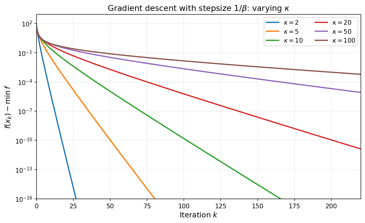
As a concrete numerical illustration, the plot below shows gradient descent with stepsize $\eta=1/\beta$ on convex quadratics with varying condition numbers, with all runs initialized at the origin. The vertical axis is $\log\bigl(f(x_k)-f^\ast\bigr)$ (shown on a semilog scale): larger $\kappa$ produces slower decay.
At this point we have extracted essentially the best guarantee available from one fixed stepsize by ensuring a contraction in every step, and then iterating the bound. The natural next question is whether coordinating multiple steps can outperform optimizing each step in isolation. The answer turns out to be yes, and leads to a dramatic improvement in iteration complexity wherein the linear dependence on $\kappa$ is replaced by a linear dependence on $\sqrt{\kappa}$.
3. Acceleration by Chebyshev Stepsizes
The analysis of gradient descent so far was quite crude in that it was based on lower-bounding the improvement in function value after $k$ iteration using a fixed step-size; in essence, the argument reduced to choosing a fixed step-size that guarantees the largest function value decrease in a single step and then iterating the bound. We now show that by monitoring performance across the entire time horizon, it is possible to choose a time-varying stepsize that yields a much faster rate of convergence. To see this, consider gradient descent with time-varying stepsizes $\eta_0, \eta_1, \ldots, \eta_{k-1}$. We saw that the error $e_j = x_j - x^\ast$ evolves as $e_{j+1} = (I - \eta_j A)\,e_j$. Therefore, after $k$ steps we have:
\[e_k = (I - \eta_{k-1}A)(I - \eta_{k-2}A)\cdots(I - \eta_0 A)\,e_0 = p_k(A)\,e_0,\]where $p_k$ is the degree-$k$ polynomial
\[p_k(\lambda) = \prod_{j=0}^{k-1}(1 - \eta_j \lambda).\]Note that we have $p_k(0) = 1$ regardless of the choice of stepsizes. Expanding $e_k$ in the eigenbasis of $A$ as before yields:
\[\begin{aligned} f(x_k) - f^\ast = \tfrac{1}{2}\|e_k\|_A^2 &= \tfrac{1}{2}\sum_{i=1}^d \lambda_i\, p_k(\lambda_i)^2\, c_i^2 \leq \max_{\lambda \in [\alpha, \beta]} p_k(\lambda)^2 \cdot \tfrac{1}{2}\|e_0\|_A^2. \end{aligned}\]Rearranging we deduce
\[\frac{f(x_k) - f^\ast}{f(x_0) - f^\ast} \leq \max_{\lambda \in [\alpha, \beta]} p_k(\lambda)^2.\]Fixed-stepsize gradient descent corresponds to the special case $p_k(\lambda) = (1 - \eta\lambda)^k$, but we are now free to choose any stepsizes. Notice that as we vary the stepsizes $\eta_0,\ldots,\eta_{k-1}$, any polynomial $p(\lambda)$ of degree at most $k$, having all real roots, and satisfying $p(0)=1$ can be realized as $p_k(\lambda)$. Thus choosing time-varying stepsizes is equivalent to choosing such a polynomial. The best possible convergence after $k$ steps is therefore determined by the minimax polynomial problem:
\[\min_{\substack{p \in \mathcal{P}^{r}_k \\ p(0) = 1}} \max_{\lambda \in [\alpha, \beta]} p(\lambda)^2. \tag{2}\]where $\mathcal{P}^r_k$ denotes the set of polynomials of degree at most $k$ with all real roots. The solution to this classical variational problem is described through so-called Chebyshev polynomials of the first kind.
Chebyshev polynomials
The Chebyshev polynomial of the first kind of degree $k$, denoted $T_k$, is defined recursively: set $T_0(x) = 1$ and $T_1(x) = x$ and define
\[T_{k+1}(x) = 2x\,T_k(x) - T_{k-1}(x) \qquad \forall k\geq 1.\]An equivalent characterization of Chebyshev polynomials is the expression
\[T_k(\cos\theta) = \cos(k\theta) \qquad \forall \theta \in [0,\pi].\]Chebyshev polynomials play a special role in numerical analysis because they solve the extremal problem:
Any degree-$k$ polynomial $p(x)$ with the same leading coefficient as $T_k$ satisfies
\[\max_{x\in [-1,1]} \lvert p(x)\rvert\geq \max_{x\in [-1,1]} \lvert T_k(x)\rvert=1.\]
In words, among all degree-$k$ polynomials with the same leading coefficient as $T_k$, the Chebyshev polynomial $T_k$ has the smallest maximum absolute value on $[-1,1]$. See the figure below that illustrates a few Chebyshev polynomial $T_k$.
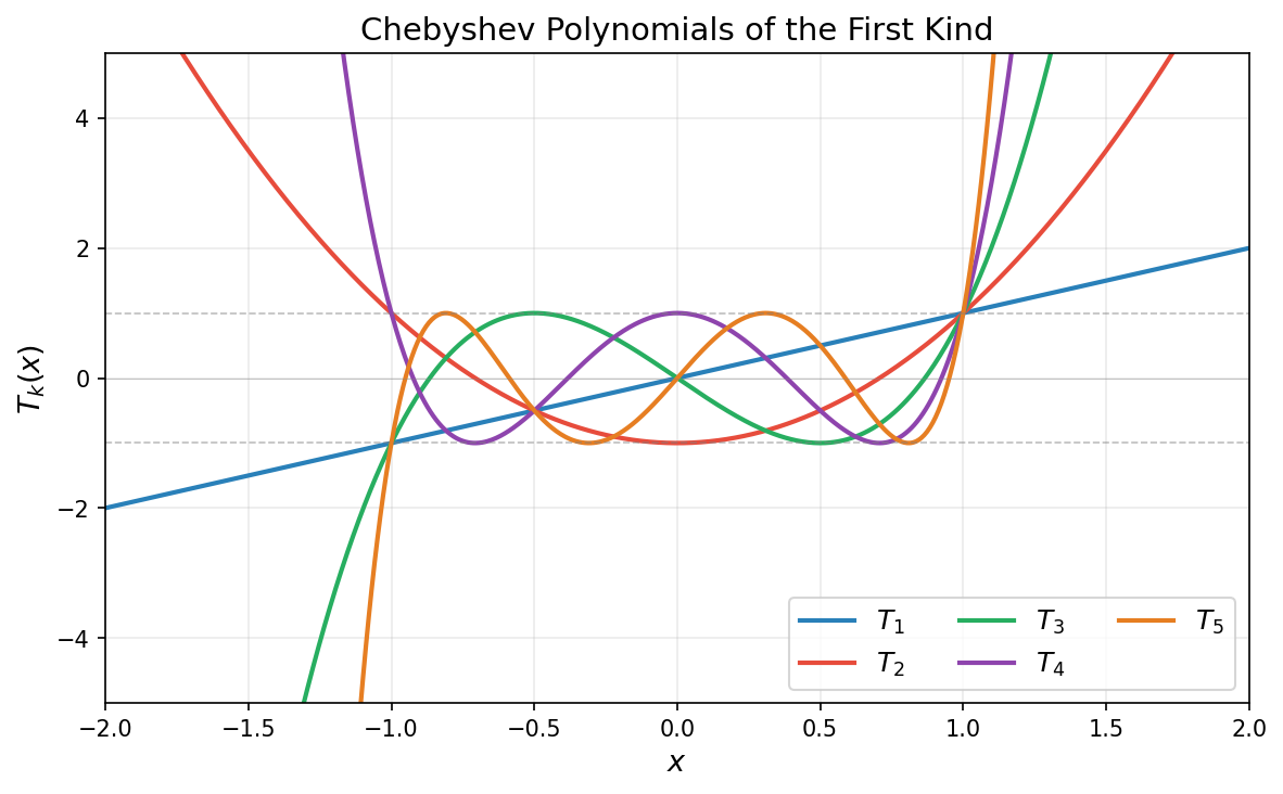
Chebyshev polynomials satisfy the following key properties:
-
Boundedness: The inequality $\lvert T_k(t)\rvert \leq 1$ holds for all $t \in [-1,1]$.
-
Roots: $T_k$ has $k$ roots in $(-1,1)$ at $t_j = \cos\left(\frac{(2j-1)\pi}{2k}\right)$ for $j = 1, \ldots, k$.
-
Explosion: For $t > 1$, we have $T_k(t) = \cosh(k\,\operatorname{arccosh}(t))$.
In summary, the Chebyshev polynomials $T_k$ are designed to be highly oscillatory on the interval $[-1,1]$ so as to stay bounded by one in absolute value, but this evidently forces these polynomials to grow rapidly outside the interval $[-1,1]$.
The optimal polynomial
Returning to gradient descent, let us see how Chebyshev polynomials yield a solution to the minimax problem $(2)$. We rescale the interval $[\alpha, \beta]$ to $[-1,1]$ with the affine change of coordinates $\varphi(\lambda)=\frac{\beta + \alpha - 2\lambda}{\beta - \alpha}$. Note that $\varphi$ sends $\lambda = 0$ to the point $\sigma := \frac{\beta + \alpha}{\beta - \alpha} = \frac{\kappa + 1}{\kappa - 1}$, assuming $\alpha>0$. Thus, under this substitution, any degree-$k$ polynomial $p(\lambda)$ with $p(0) = 1$ corresponds to a degree-$k$ polynomial $q=p\circ\varphi^{-1}$ with $q(\sigma) = 1$, and
\[\max_{\lambda \in [\alpha, \beta]}\lvert p(\lambda)\rvert = \max_{t \in [-1,1]}\lvert q(t)\rvert.\]We must therefore find the degree-$k$ polynomial $q$ with $q(\sigma) = 1$ that has the smallest maximum on $[-1,1]$. By properties 1 and 3 above, $T_k$ is bounded by $1$ on $[-1,1]$ while $T_k(\sigma) \gg 1$ for large $k$. This makes the rescaled polynomial
\[q_k^*(t):= \frac{T_k(t)}{T_k(\sigma)}\]an excellent candidate: it satisfies $q_k^{\ast}(\sigma) = 1$ and $\max_{t \in [-1,1]}\lvert q_k^{\ast}(t)\rvert = 1/T_k(\sigma)$, which is small because $T_k(\sigma)$ grows exponentially in $k$. Transforming back to the $\lambda$-variable, the optimal polynomial is
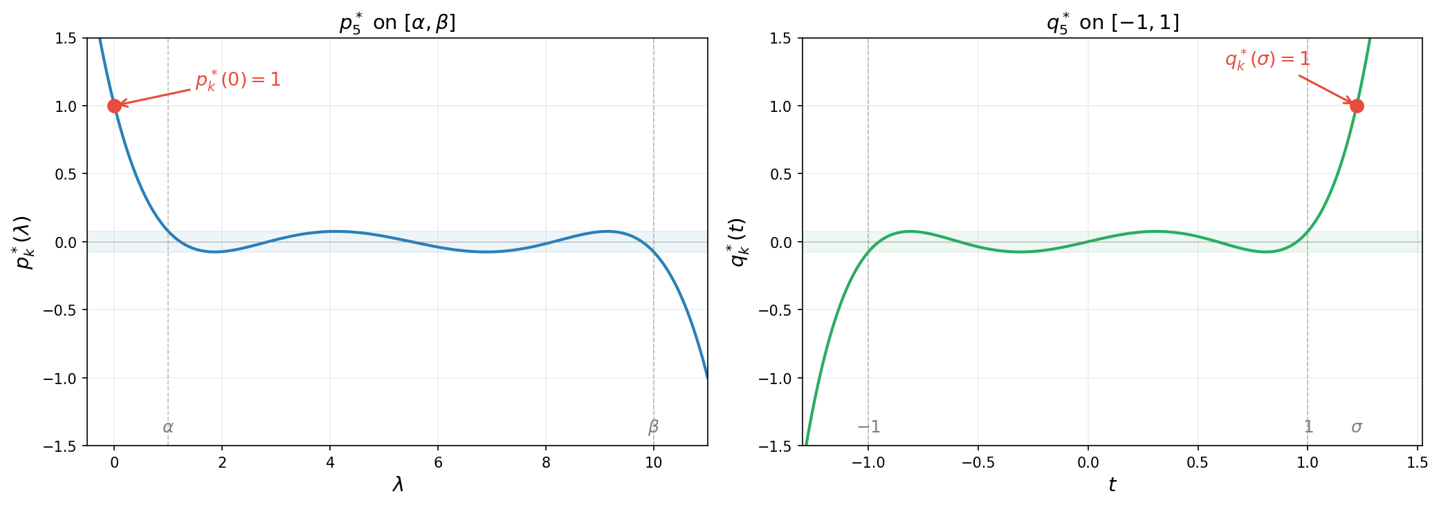
\[p_k^*(\lambda) :=(q_k^*\circ\varphi)(\lambda)= \frac{T_k\!\left(\frac{\beta + \alpha - 2\lambda}{\beta - \alpha}\right)}{T_k\!\left(\frac{\kappa + 1}{\kappa - 1}\right)}.\]Note that $p_k^*$ has all real roots. The figure below illustrates the reparametrization for $k=5$: on the left, $p_k^{\ast}$ satisfies the constraint $p_k^{\ast}(0)=1$ and oscillates with small amplitude on $[\alpha,\beta]$; on the right, $q_k^{\ast}$ satisfies $q_k^{\ast}(\sigma)=1$ and oscillates on $[-1,1]$ with the same small amplitude $1/T_k(\sigma)$.
The animation below shows $p_k^{\ast}(\lambda)$ on $[\alpha, \beta]$ for increasing degree $k$. As $k$ grows, the polynomial oscillates more rapidly yet its maximum amplitude $1/T_k(\sigma)$ shrinks exponentially—this is the mechanism behind the accelerated convergence.
Summarizing, we have the following lemma. Note that the first inequality holds as equality, as quickly follows from the extremal property of $T_k$. We omit the argument since it is not needed for what follows.
Lemma 3.1 (Chebyshev minimax). Suppose $\alpha>0$. Then with $\sigma = \frac{\kappa+1}{\kappa-1}$, the minimax value satisfies
\[\min_{\substack{p \in \mathcal{P}^r_k \\ p(0) = 1}} \max_{\lambda \in [\alpha,\beta]} \lvert p(\lambda)\rvert \leq \frac{1}{T_k(\sigma)} \leq 2\left(\frac{\sqrt{\kappa}-1}{\sqrt{\kappa}+1}\right)^k.\]Proof. We already proved the first inequality. For the second inequality, we use the identity $T_k(x) = \cosh(k\,\operatorname{arccosh}(x))$ valid for every real number $x>1$. Applying this identity with the quantity $\sigma$ gives the relation
\[\begin{aligned} \operatorname{arccosh}(\sigma) &= \ln\!\big(\sigma + \sqrt{\sigma^2 - 1}\big) = \ln\frac{\sqrt{\kappa}+1}{\sqrt{\kappa}-1}. \end{aligned}\]Consequently, the representation
\[\begin{aligned} T_k(\sigma) &= \cosh\!\left(k\ln\frac{\sqrt{\kappa}+1}{\sqrt{\kappa}-1}\right) = \frac{1}{2}\left[\left(\frac{\sqrt{\kappa}+1}{\sqrt{\kappa}-1}\right)^k + \left(\frac{\sqrt{\kappa}-1}{\sqrt{\kappa}+1}\right)^k\right] \geq \frac{1}{2}\left(\frac{\sqrt{\kappa}+1}{\sqrt{\kappa}-1}\right)^k, \end{aligned}\]holds. Taking reciprocals gives the second claim. This completes the proof. $\square$
Returning to choosing stepsizes for gradient descent, the roots of $p^{\ast}_k(\lambda)$ on $[\alpha, \beta]$ are the images of the Chebyshev roots $t_j$ under the inverse map $\varphi^{-1}(t) = \frac{\beta+\alpha}{2} - \frac{\beta-\alpha}{2}\,t$, yielding the stepsizes $\eta_j = 1/\lambda_j$. We thus have arrived at the main theorem of this section.
Theorem 3.1 (Chebyshev stepsizes). Define the stepsizes
\[\eta_j = \tfrac{1}{\lambda_j}~~ \textrm{where}~~\lambda_j = \tfrac{\beta + \alpha}{2} - \tfrac{\beta - \alpha}{2}\cos\!\left(\tfrac{(2j - 1)\pi}{2k}\right) ~~\textrm{for}~ j = 1, \ldots, k.\]Then as long as $\alpha>0$ the gradient descent iterates satisfy
\[f(x_k) - f^\ast \leq 4\left(\frac{\sqrt{\kappa} - 1}{\sqrt{\kappa} + 1}\right)^{2k}\bigl(f(x_0) - f^\ast\bigr). \tag{3}\]Proof. Combining the estimate $(2)$ and Lemma 3.1 directly yields \(\frac{f(x_k) - f^\ast}{f(x_0) - f^\ast} \leq \max_{\lambda \in [\alpha, \beta]} p_k^*(\lambda)^2 = \frac{1}{T_k(\sigma)^2}\leq 4\left(\frac{\sqrt{\kappa}-1}{\sqrt{\kappa}+1}\right)^{2k}.\) This completes the proof. $\square$
Thus, the iteration complexity of Chebyshev-accelerated gradient descent is $O(\sqrt{\kappa}\,\log((f(x_0)-f^\ast)/\varepsilon))$—a square-root improvement over the $O(\kappa\,\log((f(x_0)-f^\ast)/\varepsilon))$ complexity of fixed-stepsize gradient descent. For $\kappa = 100$, this is the difference between roughly $10$ and $100$ iterations.
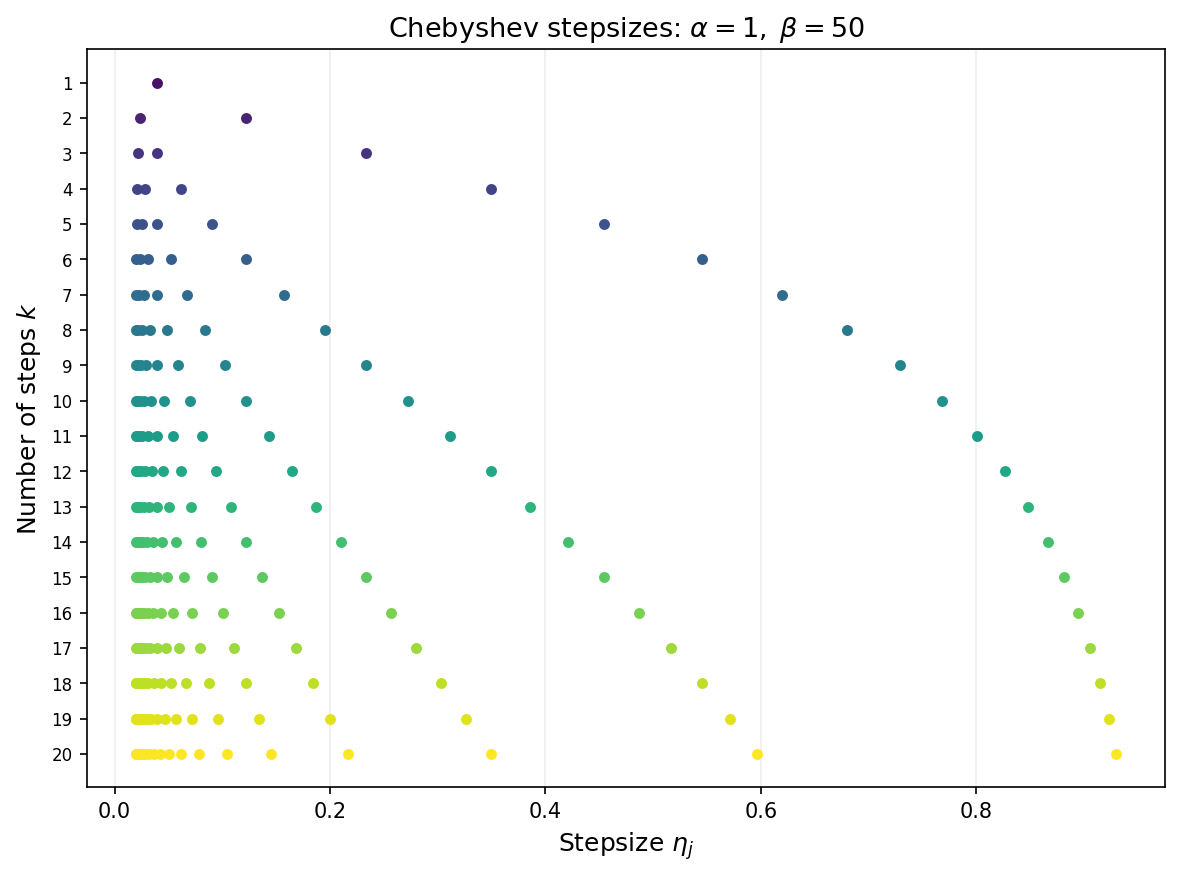
Visualizing the stepsizes and performance of the accelerated algorithm
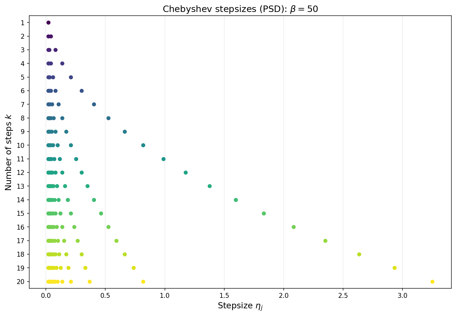
Note that the convergence guarantees are not ``anytime’’. The stepsize must be determined with the number of total iterations $k$ in mind. The next figure shows the Chebyshev stepsizes for each choice of total iteration count $k$ from 1 to 20. Each row displays the $k$ stepsizes as points along the horizontal axis. As $k$ grows, the stepsizes fill out the interval $[1/\beta,\,1/\alpha]$ with increasing density near the endpoints—reflecting the characteristic clustering of Chebyshev roots.
The animation below overlays gradient descent (blue) and Chebyshev-accelerated GD (red) on the same ill-conditioned quadratic. The Chebyshev method reaches the minimizer much faster.
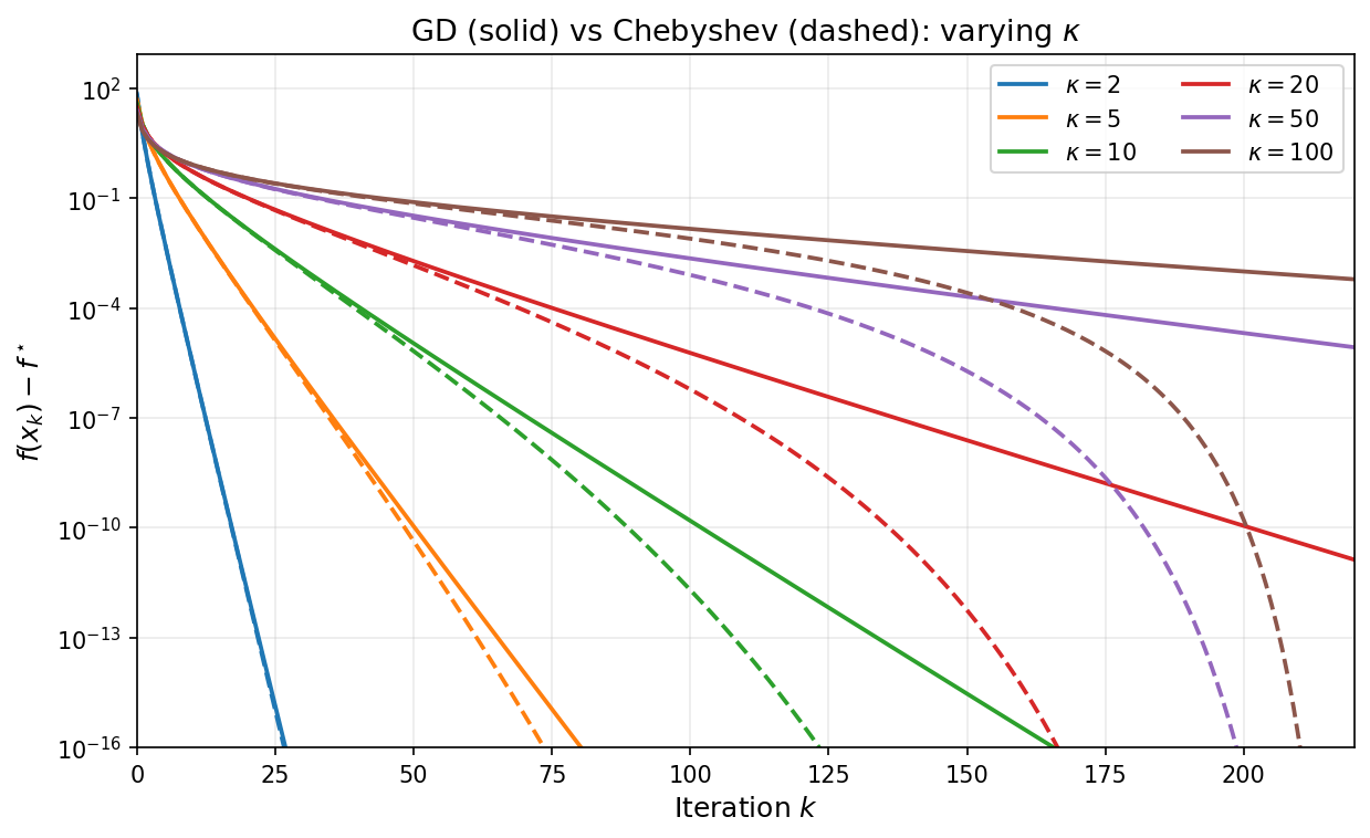
As a final illustration, the plot below overlays GD with stepsize $1/\beta$ (solid) and Chebyshev-accelerated GD with $k = 220$ (dashed) for varying condition numbers. The Chebyshev curves stay nearly flat during the cycle and then drop sharply near the final iteration, reaching machine precision much sooner than GD for every value of $\kappa$.
4. The Krylov Subspace Method and Conjugate Gradient
From polynomials to Krylov subspaces
The Chebyshev method discussed in Section 3 achieves the iteration complexity $O(\sqrt{\kappa}\,\ln((f(x_0)-f^\ast)/\varepsilon))$ by cleverly choosing time-varying stepsizes—but it requires advance knowledge of the extreme eigenvalues $\alpha$ and $\beta$. Moreover, the total number of iterations must be set in advance in order to define the stepsizes. A natural question arises:
Can we design an adaptive algorithm that matches this rate adaptively, without knowing the spectrum nor setting the time horizon?
The key observation is that gradient descent with any sequence of stepsizes produces iterates that lie in a specific linear subspace. Due to the recursion $x_{j+1} = x_j - \eta_j(Ax_j - b)$, one readily verifies the inclusion
\[x_k \in x_0 + \mathcal{K}_k(A, r_0),\]where $r_0 := b - Ax_0$ is the initial residual and
\[\mathcal{K}_k(A, r_0) := \mathrm{span}\{r_0,\, Ar_0,\, A^2 r_0,\, \ldots,\, A^{k-1}r_0\}\]is the Krylov subspace of order $k$. Both fixed-stepsize gradient descent and the Chebyshev method search within this subspace but do not fully exploit it. The natural idea is to search optimally within the Krylov subspace at each step.
The Krylov subspace method
The Krylov subspace method is the idealized algorithm that, at each step $k$, sets
\[x_k = \argmin_{x \,\in\, x_0 + \mathcal{K}_k(A,\,r_0)} f(x). \tag{4}\]It is illuminating to compare the exact performance of the Krylov method to that of gradient descent with time-varying stepsizes. Write as usual $e_0 = x_0 - x^\ast = \sum_{i=1}^d c_i v_i$ in the eigenbasis of $A$. Recall that optimizing over the stepsizes $\eta_0,\ldots,\eta_{k-1}$, yields the function-value guarantee for the last iterate of gradient descent:
\[f(x_k) - f^\ast \;=\;\min_{\substack{p \in \mathcal{P}^{r}_k \\ p(0) = 1}} \tfrac{1}{2}\sum_{i=1}^d \lambda_i\, c_i^2\, p(\lambda_i)^{2}. \tag{4a}\]For the Krylov method, any point $x \in x_0 + \mathcal{K}_k(A,r_0)$ can be written as $x = x_0 + q(A)\,r_0$ for some polynomial $q$ of degree at most $k-1$. Using the expression $r_0 = -A\,e_0$ this becomes
\[x - x^\ast \;=\; e_0 - q(A)\,A\,e_0 \;=\; p(A)\,e_0, \tag{5}\]where we define the polynomial $p(\lambda) = 1 - \lambda\,q(\lambda)$. As $q$ varies over polynomials of degree at most $k-1$, the polynomial $p$ varies over all of $\mathcal{P}_k$ with $p(0)=1$, with no real-root restriction. The defining property $(4)$ therefore yields the equality
\[f(x_k) - f^\ast \;=\; \min_{\substack{p \in \mathcal{P}_k \\ p(0) = 1}} \tfrac{1}{2}\sum_{i=1}^d \lambda_i\, c_i^2\, p(\lambda_i)^{2}\qquad \forall k. \tag{4b}\]The two expressions $(4a)$ and $(4b)$ differ in exactly one formal respect: the Krylov method optimizes over all polynomials with $p(0)=1$, whereas gradient descent is confined to those with real roots.
Theorem 4.1 (Krylov method convergence). Assuming $\alpha > 0$, the Krylov subspace method $(4)$ satisfies
\[f(x_k) - f^\ast \leq 4\left(\frac{\sqrt{\kappa} - 1}{\sqrt{\kappa} + 1}\right)^{2k}\bigl(f(x_0) - f^\ast\bigr) \qquad \forall k\geq 0.\]Moreover, the method converges in at most $m$ iterations, where $m$ is the number of distinct eigenvalues of $A$.
Proof. The linear rate follows directly from Theorem $3.1$: the $k$th iterate produced by the Chebyshev stepsizes lies in $x_0+\mathcal{K}_k(A,r_0)$, whereas the Krylov method minimizes $f$ over that entire affine space, and so cannot do worse.
To prove finite termination, observe that by $(4b)$ it suffices to exhibit a polynomial $p \in \mathcal{P}_m$ with $p(0)=1$ for which $\sum_{i=1}^d \lambda_i\,c_i^2\,p(\lambda_i)^2 = 0$, since this forces $f(x_m) = f^\ast$ and hence $x_m = x^\ast$. Take
\[p(\lambda):=\prod_{i=1}^m\left(1-\frac{\lambda}{\lambda_i}\right),\]where $\lambda_1,\ldots,\lambda_m$ are the distinct eigenvalues of $A$. Then $p$ has degree $m$, satisfies $p(0)=1$, and vanishes at every eigenvalue of $A$, so the sum is zero as required. $\square$
The convergence bound in Theorem 4.1 is identical to the Chebyshev bound in Theorem 3.1, and the iteration complexity has the same order $O(\sqrt{\kappa}\,\ln((f(x_0)-f^\ast)/\varepsilon))$. Importantly, the Krylov method achieves this complexity without knowing $\alpha$ or $\beta$ and without requiring to specify the time horizon $k$; moreover, finite termination provides an absolute guarantee of at most $m$ steps, where $m$ is the number of distinct eigenvalues. In practice, clustered eigenvalues lead to far fewer iterations than the worst-case bound suggests.
The Conjugate Gradient algorithm implements the Krylov method
The Krylov subspace method $(4)$ is conceptual: a direct implementation would solve a $k$-dimensional linear optimization problem at each step, with cost growing as $k$ increases. The Conjugate Gradient (CG) algorithm is an implementation of the Krylov method that uses only one matrix-vector product per iteration.
The key idea is to iteratively build a basis of the Krylov subspaces that is orthogonal with respect to the inner product $\langle x,y\rangle_A=x^\top Ay$, so that each successive minimization reduces to a single line search. Conceptually, this basis is formed by a Gram–Schmidt process. The special structure of Krylov subspaces ensures that each Gram–Schmidt update requires only the immediately preceding direction—a short recurrence—rather than all previous directions.
Concretely, suppose that we have constructed an $A$-orthogonal basis $\lbrace p_i\rbrace _{i=0}^{k-1}$ for $\mathcal{K}_{k}$ and that we have available a minimizer $x_k$ of $f$ on $x_0 + \mathcal{K}_k$. Let us see how we can efficiently extend the $A$-orthogonal basis to $\mathcal{K}_{k}$ and construct the minimizer $x_{k+1}$ of $f$ on $x_0 + \mathcal{K}_{k+1}$. To this end, define the residuals $$r_i=-\nabla f(x_i)=b-Ax_i.$$
Observe that we may write $r_k=b-Ax_k=r_0-A(x_k-x_0)$ and therefore $r_k$ lies in $\mathcal{K}_{k+1}$. Now, set $$p_{k}=r_k+\beta_{k-1} p_{k-1},$$ for a constant $\beta_{k-1}$ to be chosen. We would like to ensure that $p_{k}$ is $A$-orthogonal to $\lbrace p_i\rbrace _{i=0}^{k-1}$ . To this end, setting $p_{k}^\top Ap_{k-1}=0$ yields the unique choice of $\beta_{k-1}=-\frac{r_k^\top Ap_{k-1}}{p_{k-1}^\top Ap_{k-1}}$. Now for any $i<k-1$ we compute $$p_{k}^{\top}A p_{i}=r_k^\top A p_{i}+\beta_{k-1}p_{k-1}^{\top}Ap_i.$$ Observe that $p_{k-1}^{\top}Ap_i=0$ by assumed A-orthogonality of $\lbrace p_i\rbrace _{i=0}^{k-1}$ and $r_k^\top A p_{i}=0$ because $A p_{i}$ lies in $\mathcal{K}_{i+1}$ and the optimality conditions for $x_k$ imply $r_k\perp K_{k}$. Thus $\lbrace p_i\rbrace _{i=0}^{k}$ is indeed an A-orthogonal basis for $\mathcal{K}_{k}$. It remains to declare $$x_{k+1}=\argmin_{\eta} f(x_k+\eta p_{k}). \tag{6}$$Indeed, taking the derivative in $\eta$ implies $r_{k+1}\perp p_{k}$ and for any $i<k$ we have orthogonality $$r_{k+1}^\top p_{i}=(r_k-\eta_k Ap_k)^{\top}p_i=r_k^\top p_i-\eta_k p_k^\top Ap_i=0,$$ where $\eta_k$ is the minimizer of $(6)$. Thus $x_{k+1}$ is indeed the minimizer of $f$ on $x_0+\mathcal{K}_{k+1}$. The algorithm we just constructed is called the conjugate gradient method and is summarized in the following.
Algorithm 1 (Conjugate Gradient Method)
Input: $x_0 \in \mathbb{R}^d$
- Set $r_0 = b - Ax_0$, $\;p_0 = r_0$
- For $k = 0, 1, 2, \ldots$ do:
- $\qquad \eta_k = \dfrac{r_k^\top r_k}{p_k^\top A p_k}$
- $\qquad x_{k+1} = x_k + \eta_k\, p_k$
- $\qquad r_{k+1} = r_k - \eta_k\, A p_k$
- $\qquad \beta_k = -\dfrac{r_{k+1}^\top A p_k}{p_k^\top A p_k}$
- $\qquad p_{k+1} = r_{k+1} + \beta_k\, p_k$
Each iteration of the conjugate gradient method requires one matrix-vector product $Ap_k$, the same per-step cost as gradient descent. The vectors $r_k = b - Ax_k$ are the residuals satisfying $r_k = -\nabla f(x_k)$, while the vectors $p_k$ are the search directions. The stepsize $\eta_k$ minimizes $f$ along the ray $x_k + \eta\, p_k$, while $\beta_k$ ensures $A$-orthogonality of consecutive search directions.
Remark. In the literature, the update for $\beta_k$ is usually written in the equivalent form $\beta_k = \lVert r_{k+1}\rVert ^2/\lVert r_k\rVert ^2$. The equivalence is straightforward to establish from the residual recursion $Ap_k = (r_k - r_{k+1})/\eta_k$; we omit the argument for brevity.
Visualizing CG
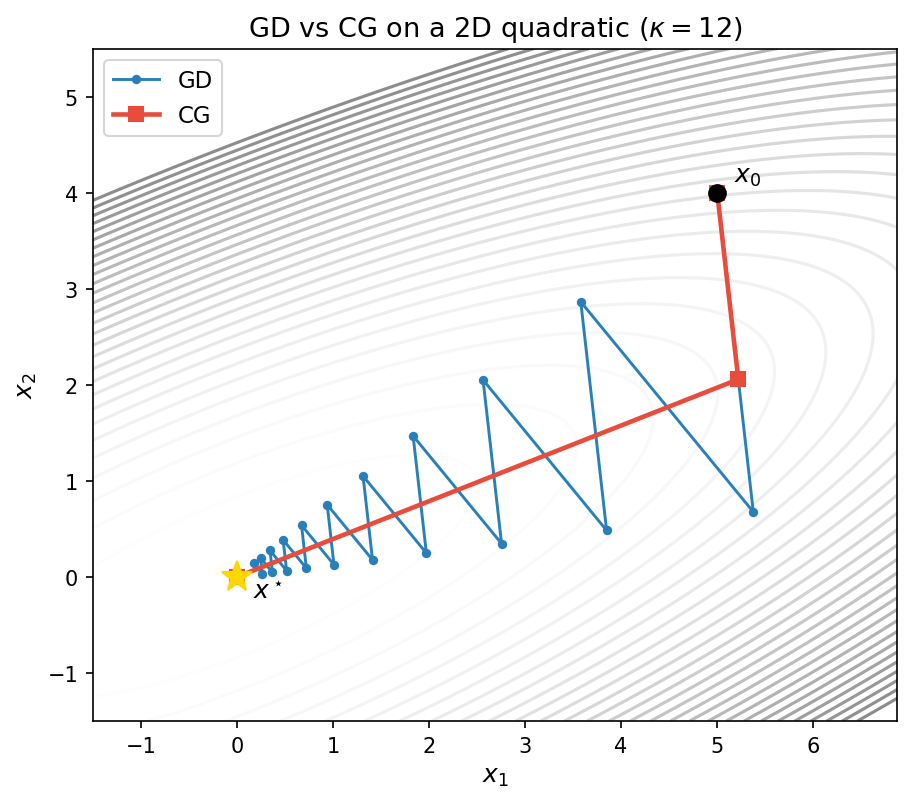
The figure below compares GD and CG on the same ill-conditioned 2D quadratic ($\kappa = 12$). Gradient descent (blue) zig-zags along the narrow valley, requiring many iterations to approach the minimum. CG (red) reaches the minimum in exactly 2 steps—the dimension of the problem—by choosing $A$-orthogonal search directions that span the full space.
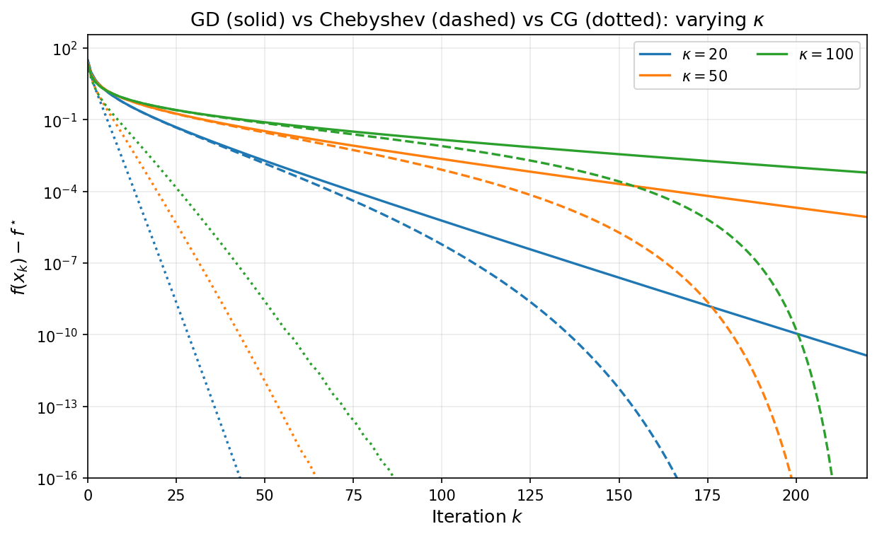
The next figure repeats the varying-$\kappa$ experiment from Section 3, now with CG (dotted) added alongside GD (solid) and Chebyshev (dashed). For each condition number, CG converges much faster than gradient descent and the Chebyshev method—without requiring knowledge of $\alpha$ or $\beta$, and without presetting the number of iterations.
6. Sublinear Rates in the Positive Semidefinite Case
Motivation
The convergence guarantees of the previous sections all rely on the assumption $\alpha > 0$—that is, $A$ is positive definite. When $\alpha$ is very close to zero, however, the condition number $\kappa = \beta/\alpha$ can become arbitrarily large and the linear convergence bounds of Theorems 1, 2, and 3 essentially become vacuous. This situation arises often in practice. As a concrete example let us look at the prototypical problem of solving a linear system generated by a kernel matrix.
Example (Kernel matrices and spectral decay). A kernel function $k\colon\mathbb{R}^d\times\mathbb{R}^d\to\mathbb{R}$ is a symmetric function such that the kernel matrix $K\in\mathbb{R}^{n\times n}$ defined by $K_{ij}=k(x_i,x_j)$ is positive semidefinite for every finite collection of points $x_1,\dots,x_n\in\mathbb{R}^d$. Kernel matrices are ubiquitous: they arise in Gaussian process regression, support vector machines, kernel ridge regression, and radial-basis-function interpolation. Given a target vector $y\in\mathbb{R}^n$, the core computational task reduces to solving the linear system
\[K\alpha = y,\]which is exactly the quadratic minimization problem $\min_\alpha \tfrac{1}{2}\alpha^\top K\alpha - y^\top \alpha$.
Two of the most widely used kernels depend only on the $\ell_2$ distance $\lVert x-y\rVert $ and a length-scale parameter $\sigma>0$, called the bandwidth. The Gaussian (RBF) kernel is
\[k_{\mathrm{RBF}}(x,y)=\exp\!\left(-\frac{\|x-y\|^2}{2\sigma^2}\right).\]It is infinitely differentiable ($C^\infty$). The Laplace kernel is \(k_{\mathrm{Lap}}(x,y)=\exp\!\left(-\frac{\|x-y\|}{\sigma}\right).\) It is continuous but not differentiable at the origin ($C^0$). The Laplace kernel is the Matérn kernel with $m=\tfrac12$. More generally, the Matérn family interpolates between Laplace and Gaussian by introducing a smoothness parameter $m>0$. The general Matérn kernel is
\[k_m(x,y)=\frac{2^{1-m}}{\Gamma(m)}\left(\frac{\sqrt{2m}\,\|x-y\|}{\sigma}\right)^m K_m\!\left(\frac{\sqrt{2m}\,\|x-y\|}{\sigma}\right),\]where $K_m$ is the modified Bessel function of the second kind. The parameter $m$ controls the smoothness: the Matérn kernel with parameter $m$ is $\lceil m\rceil -1$ times continuously differentiable. Several important finite-$m$ cases, together with the Gaussian limit, are summarized in the following table:
| Kernel | $m$ | Closed form | Smoothness |
|---|---|---|---|
| Laplace | $\tfrac12$ | $\exp\bigl(-\tfrac{\lVert x-y\rVert }{\sigma}\bigr)$ | $C^0$ |
| Matérn 3/2 | $\tfrac32$ | $\bigl(1+\tfrac{\sqrt{3}\lVert x-y\rVert }{\sigma}\bigr)\exp\bigl(-\tfrac{\sqrt{3}\lVert x-y\rVert }{\sigma}\bigr)$ | $C^1$ |
| Matérn 5/2 | $\tfrac52$ | $\bigl(1+\tfrac{\sqrt{5}\lVert x-y\rVert }{\sigma}+\tfrac{5\lVert x-y\rVert ^2}{3\sigma^2}\bigr)\exp\bigl(-\tfrac{\sqrt{5}\lVert x-y\rVert }{\sigma}\bigr)$ | $C^2$ |
| Gaussian (RBF) | $\infty$ | $\exp\bigl(-\tfrac{\lVert x-y\rVert ^2}{2\sigma^2}\bigr)$ | $C^\infty$ |
In the limit $m\to\infty$ the Matérn kernel recovers the Gaussian kernel.
For reasonable distributions of data points (e.g., Gaussian, uniform, or with a bounded density on a compact set), the eigenvalues of the normalized kernel matrix $(1/n)K$ resemble those of an associated linear integral operator, whose spectral decay can be analyzed explicitly. More precisely suppose that the points $x_1,\ldots, x_n$ are drawn iid from a distribution $\nu$ on $\mathbb{R}^d$. For any function $f\in L_2(\nu)$ define the $n$-dimensional vector
\[f^{(n)}=\tfrac{1}{\sqrt{n}}(f(x_1),\ldots, f(x_n)).\]Then we may write the quadratic form of $\frac{1}{n}K$ as
\[(f^{(n)})^\top (\tfrac{1}{n}K)(f^{(n)})=\frac{1}{n^2}\sum_{i,j}k(x_i,x_j)f(x_i)f(x_j)=\int\int k(x,x')f(x)f(x')~dP_n(x)dP_n(x'),\]where $dP_n=\frac{1}{n}\sum_{i=1}^n\delta_{x_i}$ is the atomic measure on the samples. As $n$ tends to infinity, under mild assumptions, the right-hand-side tends to the integral quadratic form $T\colon L_2(\nu)\times L_2(\nu)\to \mathbb{R}$ given by
\[T(f,f)=\int\int k(x,x')f(x)f(x')~d\nu(x)d\nu(x').\]Note that this quadratic form is generated by the linear operator on functions $T\colon L_2(\nu)\to L_2(\nu)$ given by
\[(Tf)(x)=\int k(x,x')f(x')\,d\nu(x').\]Heuristically, in the large-sample limit the eigenvalues of $\tfrac{1}{n}K$ approximate those of the integral operator $T$. Let $\mu_1\geq\mu_2\geq\cdots$ denote the eigenvalues of $T$, and let $p$ denote the intrinsic dimension of the data support. The end result is the following asymptotic estimate that holds for all sufficiently large eigenvalue indices $i$:
| Kernel | Eigenvalue decay | Rate for $\mu_i$ |
|---|---|---|
| Laplace ($m=\tfrac12$) | polynomial | $\mu_i\asymp i^{-(1+p)/p}$ |
| Matérn (smoothness $m$) | polynomial | $\mu_i\asymp i^{-(2m+p)/p}$ |
| Gaussian (RBF) | super-exponential | $\mu_i\lesssim C\exp(-c\, i^{2/p})$ |
As a consequence, kernel matrices are typically extremely ill-conditioned: the effective condition number $\lambda_1/\lambda_n$ grows rapidly with $n$, and for large $n$ many eigenvalues are numerically zero. This is precisely the regime where the positive definite theory becomes vacuous.
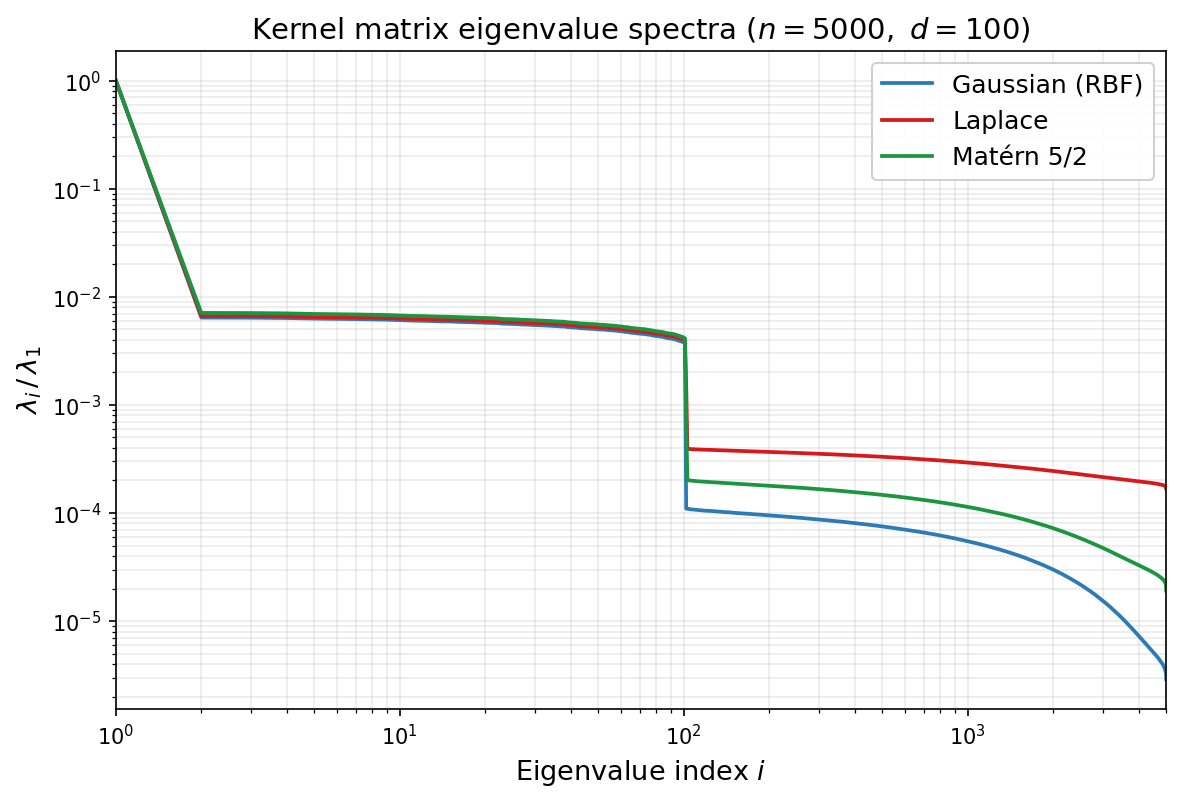
The figure below illustrates this phenomenon on synthetic data. We draw $n=5000$ points independently from the standard Gaussian distribution $\mathcal{N}(0,I_{100})$ in $\mathbb{R}^{100}$, use the same sample for all three kernels, choose the bandwidth $\sigma$ by the median heuristic, and plot the normalized eigenvalues $\lambda_i/\lambda_1$ on a log-log scale. A noticeable bend appears around index $i\approx d=100$; this is a finite-sample crossover caused by the interaction between the ambient dimension, the sampling distribution, and the kernel bandwidth, rather than a direct prediction of the asymptotic estimates above. The asymptotic theory instead describes the tail behavior after such pre-asymptotic effects: past the bend, the three kernels separate clearly. The Gaussian kernel (blue) exhibits the fastest decay, the Laplace kernel (red) the slowest, and the Matérn 5/2 kernel (green) is intermediate, in qualitative agreement with the rates in the table.
We will now develop convergence guarantees for all of the methods we have seen—gradient descent, Chebyshev-accelerated gradient descent, and the Krylov method—that are insensitive to the minimal eigenvalue of $A$. The price to pay is that the logarithmic dependence on $1/\varepsilon$ in the positive definite case degrades to a polynomial dependence on $1/\varepsilon$.
Setup
We consider the same quadratic objective $f(x) = \tfrac{1}{2}x^\top Ax - b^\top x$, but now we allow $\alpha = 0$. We assume throughout that $b \in \mathrm{range}(A)$, ensuring that the solution set
\[S = \{x \in \mathbb{R}^d : Ax = b\}\]is nonempty and we let $x^{\ast}\in S$ be arbitrary.
The eigenvalues of $A$ are ordered as
\[0 = \lambda_1 = \cdots = \lambda_r < \lambda_{r+1} \leq \cdots \leq \lambda_d = \beta,\]where $r \geq 1$ is the dimension of $\ker(A)$.
Gradient descent
We begin with the convergence rate of gradient descent. The key idea is that we have previously shown the exact relation \(f(x_k) - f^\ast = \frac{1}{2}\sum_{i=1}^{d}\lambda_i(1-\eta\lambda_i)^{2k}\,c_i^2\) where $\eta$ is the stepsize and $c_i$ are the coefficients of the initial error in the eigenbasis of $A$. Previously, we pulled out $\sup_{\lambda\in [\alpha,\beta]}(1-\eta\lambda)^{2k}$ from the sum. We now instead pull out $\sup_{\lambda\in [\alpha,\beta]}\lambda(1-\eta\lambda)^{2k}$.
Theorem 6.1 (Sublinear convergence of gradient descent). With stepsize $\eta = 1/\beta$, the gradient descent iterates satisfy
\[f(x_k) - f^\ast \leq \frac{\beta}{2(2k+1)}\,\|x_0 - x^\ast\|^2 \tag{7}.\]Proof. Writing out the initial error $e_0=x_0-x^\ast=\sum_{i=1}^d c_i v_i$ in the eigen-basis of $A$ yields
\[f(x_k) - f^\ast = \frac{1}{2}\sum_{i=1}^{d}\lambda_i(1-\lambda_i/\beta)^{2k}\,c_i^2 \leq \frac{1}{2}\max_{\lambda \in [0,\beta]}\lambda(1-\lambda/\beta)^{2k}\cdot\|e_0\|^2.\]Elementary calculus shows $\sup_{t\in [0,1]}t(1-t)^{q}=\frac{1}{1+q}(\frac{q}{1+q})^q\leq \frac{1}{1+q}$. Therefore setting $q=2k$ yields
\[\max_{\lambda \in (0,\beta]}\lambda(1-\lambda/\beta)^{2k} \leq \frac{\beta}{2k+1},\]which completes the proof. $\square$
From Theorem 6.1, converting to complexity, the bound $f(x_k) - f^\ast \leq \varepsilon$ is guaranteed to hold whenever
\[k \geq \frac{\beta\,\|x_0 - x^\ast\|^2}{4\varepsilon}.\]Thus the iteration complexity is
\[O\!\left(\frac{\beta\,\|x_0 - x^\ast\|^2}{\varepsilon}\right).\]Compared with the $O(\kappa\,\ln(1/\varepsilon))$ complexity of gradient descent in the positive definite case, the dependence on accuracy has changed from logarithmic to polynomial: achieving an additional digit of accuracy now requires a tenfold increase in iterations, rather than a fixed additive cost. This is the hallmark of sublinear convergence.
Note that an important feature of Theorem 6.1 is that the convergence bound involves the squared Euclidean distance $\lVert x_0 - x^\ast\rVert ^2$ rather than the initial function gap $f(x_0) - f^\ast$, and this is unavoidable.
Acceleration by Chebyshev stepsizes
As in the positive definite case, the $O(1/k)$ rate of fixed-stepsize gradient descent can be improved by varying the stepsize across iterations. Recall that the Chebyshev stepsizes arose in the positive definite case from the fact that the Chebyshev polynomial of the first kind $T_k$ minimizes $\max_{\lambda \in [-1,1]} p(\lambda)^2$ over all degree at most $k$ polynomials with the same leading coefficient. In the positive semidefinite case, the Chebyshev polynomials of the second kind will play an analogous role.
Chebyshev polynomials of the second kind
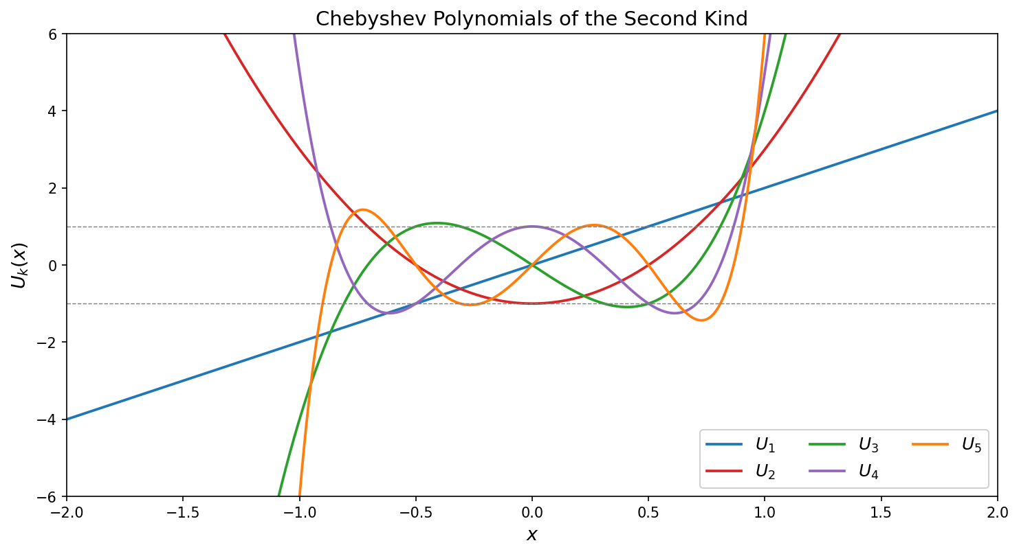
Chebyshev polynomials of the second kind are defined by the same recurrence as $T_k$ but with a different initial condition: set $U_0(x) = 1$ and $U_1(x) = 2x$ and define
\[U_{j+1}(x) = 2x\,U_j(x) - U_{j-1}(x) \qquad \forall j\geq 1.\]An equivalent trigonometric characterization is
\[U_j(\cos\theta) = \frac{\sin\bigl((j+1)\theta\bigr)}{\sin\theta},\]from which one directly sees $U_j(1) = j+1$. See the figure below.
The Chebyshev polynomials of the second kind solve a weighted analogue of the extremal problem for $T_k$:
Any degree-$k$ polynomial $p(x)$ with the same leading coefficient as $U_k$ satisfies
\[\max_{x\in [-1,1]} \sqrt{1-x^2}\,\lvert p(x)\rvert\geq \max_{x\in [-1,1]} \sqrt{1-x^2}\,\lvert U_k(x)\rvert=1.\]
The equality on the right follows from the identity $\sqrt{1-x^2}\,U_k(x) = \sin((k+1)\theta)$ when $x=\cos\theta$. As we will see, the weight $\sqrt{1-x^2}$ is precisely what arises from the extra factor of $\lambda$ in the PSD minimax problem after the change of variables.
The key properties, paralleling those of $T_k$, are:
- Boundedness: $\lvert U_k(\cos\theta)\rvert \leq k+1$ for all $\theta$, and moreover $\lvert \sin\theta\, U_k(\cos\theta)\rvert = \lvert\sin((k+1)\theta)\rvert \leq 1$.
- Roots: $U_{k}$ has $k$ roots in $(-1,1)$ at $\cos(j\pi/(k+1))$ for $j = 1, \ldots, k$.
- Growth at edges: $U_k(1) = k+1$, so $U_k$ grows polynomially at $x=1$, in contrast to the exponential growth of $T_k$.
We now linearly reparametrize and rescale the $U_{k-1}$ and define \(\phi_k(\lambda) = \left(1 - \frac{\lambda}{\beta}\right)\frac{U_{k-1}(1 - 2\lambda/\beta)}{k}.\) Note that we have $\phi_k(0) = 1$ and the roots of $\phi_k$ on $[0,\beta]$ are $\lambda_j = \beta\sin^2(j\pi/(2k))$ for $j = 1, \ldots, k$.
Lemma 6.2 (Chebyshev minimax, PSD case). The polynomial $\phi_k$ satisfies
\[\max_{\lambda \in [0,\beta]}\,\lambda\,\phi_k(\lambda)^2 \leq \frac{\beta}{4k^2}. \tag{10}\]Proof. Substitute $\cos\theta = 1 - 2\lambda/\beta$ for $\theta \in [0,\pi]$, so that $\lambda = \beta\sin^2(\theta/2)$ and $1 - \lambda/\beta = \cos^2(\theta/2)$. The Chebyshev identity gives $U_{k-1}(\cos\theta) = \sin(k\theta)/\sin\theta$, and the factorization $\sin\theta = 2\sin(\theta/2)\cos(\theta/2)$ yields
\[\begin{aligned} \lambda\,\phi_k(\lambda)^2 &= \beta\sin^2(\theta/2)\cdot\cos^4(\theta/2)\cdot\frac{\sin^2(k\theta)}{k^2\sin^2\theta} \\[4pt] &= \beta\sin^2(\theta/2)\cdot\cos^4(\theta/2)\cdot\frac{\sin^2(k\theta)}{4k^2\sin^2(\theta/2)\cos^2(\theta/2)} \\[4pt] &= \frac{\beta\cos^2(\theta/2)\,\sin^2(k\theta)}{4k^2}. \end{aligned}\]Since $\cos^2(\theta/2) \leq 1$ and $\sin^2(k\theta) \leq 1$ for all $\theta$, the claim follows. $\square$
We are now ready to see the accelerated rate.
Theorem 6.2 (Chebyshev stepsizes, PSD case). Define the stepsizes
\[\eta_j = \frac{1}{\beta\sin^2(j\pi/(2k))} \qquad \textrm{for}~ j = 1, \ldots, k.\]Then the gradient descent iterates satisfy
\[f(x_k) - f^\ast \leq \frac{\beta}{8k^2}\,\|x_0 - x^\ast\|^2. \tag{9}\]Proof. Write the initial error in the eigenbasis of $A$ as $ e_0=x_0-x^\ast=\sum_{i=1}^d c_i v_i. $ For gradient descent with stepsizes $\eta_1,\dots,\eta_k$, define the degree-$k$ polynomial $ p_k(\lambda):=\prod_{j=1}^k(1-\eta_j\lambda). $ By the choice $ \eta_j = \frac{1}{\beta\sin^2(j\pi/(2k))} $ we have $ p_k(\lambda)=\phi_k(\lambda). $ Therefore, the general error formula from Section 2 gives \(f(x_k) - f^\ast = \tfrac{1}{2}\sum_{i=1}^d \lambda_i\, \phi_k(\lambda_i)^2\, c_i^2 \leq \tfrac{1}{2}\max_{\lambda \in [0,\beta]} \lambda\,\phi_k(\lambda)^2 \sum_{i=1}^d c_i^2.\) Applying Lemma 6.2 and using $\sum_{i=1}^d c_i^2=\lVert e_0\rVert ^2=\lVert x_0-x^\ast\rVert ^2$, we obtain \(f(x_k) - f^\ast \leq \tfrac{1}{2}\cdot\frac{\beta}{4k^2}\cdot\|x_0-x^\ast\|^2 = \frac{\beta}{8k^2}\,\|x_0 - x^\ast\|^2.\) This completes the proof. $\square$
Thus, the iteration complexity of the Chebyshev accelerated algorithm is $O(\sqrt{\beta\,\lVert x_0 - x^\ast\rVert ^2/\varepsilon})$—a square-root improvement over the $O(\beta\,\lVert x_0 - x^\ast\rVert ^2/\varepsilon)$ complexity of fixed-stepsize gradient descent. This is a quadratic improvement in the complexity.
The corresponding stepsize schedule in the positive semidefinite case is shown below for several values of $k$.
As in the positive definite case, the Chebyshev stepsizes require knowledge of $\beta$ and the total number of iterations $k$ must be fixed in advance.
Conjugate gradient in the positive semidefinite case
The Krylov subspace method in the PSD setting is defined exactly as before: at step $k$, it minimizes $f$ over the affine space \(x_0+\mathcal{K}_k(A,r_0).\) The only new issue is that $A$ may be singular. However, since $b\in\mathrm{range}(A)$ and $Ax_0\in\mathrm{range}(A)$, the residual $ r_0=b-Ax_0 $ lies in $\mathrm{range}(A)$. Therefore the entire Krylov subspace $\mathcal{K}_k(A,r_0)$ is contained in $\mathrm{range}(A)$, and $A$ is positive definite on that subspace. Consequently, the same short-recurrence argument from Section 4 shows that, until termination, the conjugate gradient method is well-defined and implements the PSD Krylov method: at each step, the CG iterate $x_k$ minimizes $f$ over $x_0+\mathcal{K}_k(A,r_0)$. With this observation in hand, the convergence analysis is immediate from Theorem 6.2, exactly as in the positive definite case.
Theorem 6.3 (CG convergence, PSD case). The CG iterates satisfy
\[f(x_k) - f^\ast \leq \frac{\beta}{8k^2}\,\|x_0 - x^\ast\|^2, \tag{11}\]and CG terminates in at most $m$ iterations, where $m$ is the number of distinct nonzero eigenvalues of $A$.
Proof. The rate follows directly from Theorem 6.2: the $k$th iterate produced by the PSD Chebyshev stepsizes lies in $x_0+\mathcal{K}_k(A,r_0)$, whereas CG minimizes $f$ over that entire affine space and so cannot do worse. $\square$
The bound $(11)$ matches the PSD Chebyshev bound $(9)$; the gain of CG is that it attains this behavior adaptively, without requiring $\beta$ or a preset horizon.
Numerical illustration
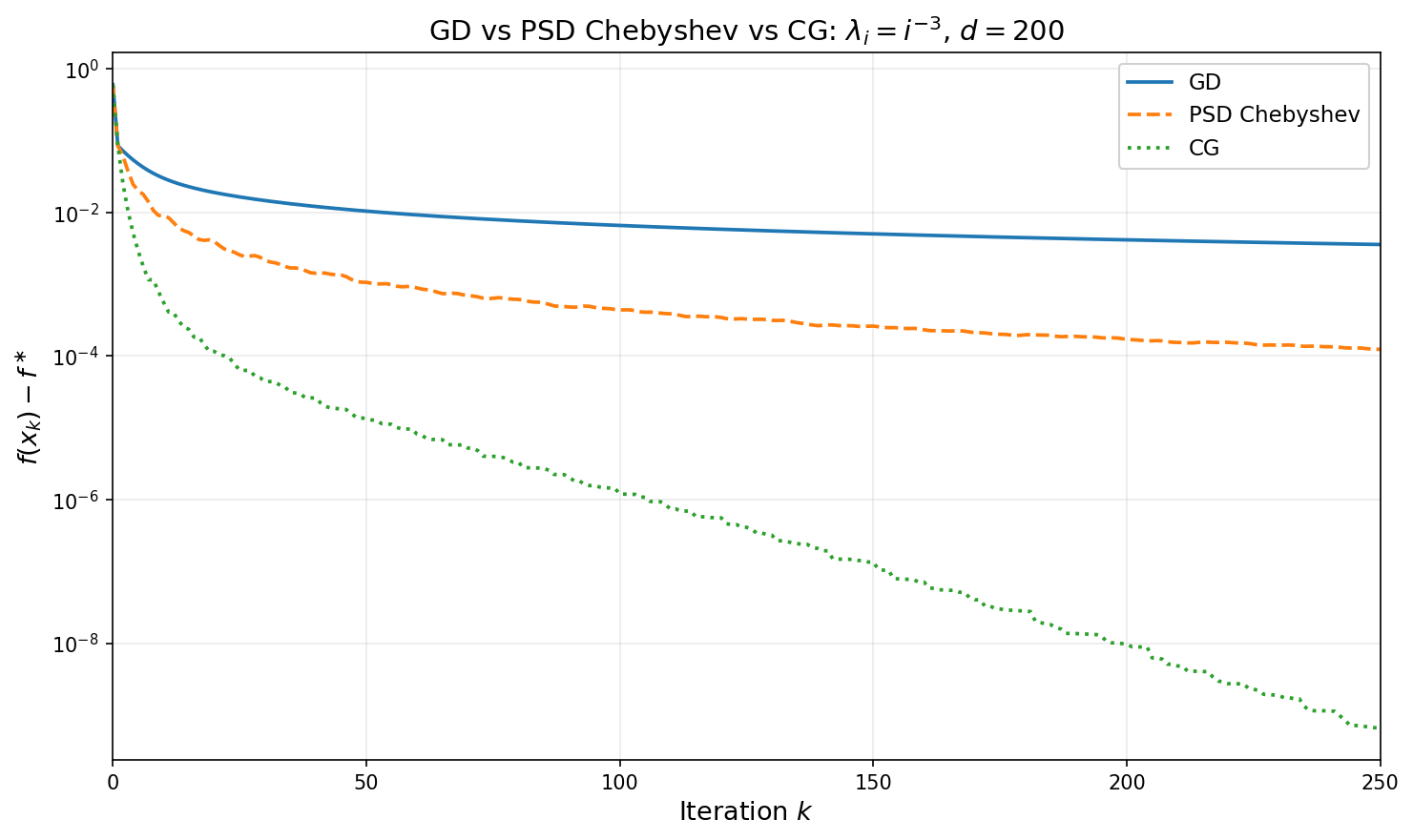
The figure below compares GD, PSD Chebyshev, and CG on a $d=200$ dimensional quadratic whose spectrum follows the power law $\lambda_i = i^{-3}$ (condition number $\approx 8\times 10^6$). For each horizon $k$, the PSD Chebyshev point plotted is the iterate after running all $k$ stepsizes from $x_0$. The sublinear separation between GD ($O(1/k)$) and Chebyshev ($O(1/k^2)$) is clearly visible, while CG reaches high accuracy in far fewer iterations.
7. Convergence Under Source Conditions and Spectral Structure
Beyond worst-case analysis
Up to this point, we emphasized worst-case bounds obtained from extreme eigenvalues alone. In this section, we obtain refined and improved guarantees that take into account the entire spectrum of the matrix $A$, rather than its extreme eigenvalues. These refined bounds are important in practice because in high-dimensional problems, the distribution of eigenvalues is often far from the worst case, and exploiting this structure leads to substantially sharper estimates.
As motivation, recall from Section 4 that the conjugate gradient method satisfies the exact error formula
\[f(x_k) - f^\ast \;=\; \min_{\substack{p \in \mathcal{P}_k \\ p(0)=1}}\, \frac{1}{2}\sum_{i=1}^d \lambda_i\,p(\lambda_i)^{2}\,c_i^2, \tag{12}\]where $c_i$ are the coefficients of $e_0 = x_0 - x^\ast$ in the eigenbasis of $A$. The worst-case analysis upper bounds this minimum by exhibiting a particular polynomial $p$ — a (shifted) Chebyshev polynomial — and then bounding the resulting sum by pulling out the maximum: $\max_{\lambda\in[\alpha,\beta]} p(\lambda)^2$ in the positive definite case, or $\max_{\lambda\in[0,\beta]} \lambda\, p(\lambda)^2$ in the positive semidefinite case. This bound ignores two sources of structure:
-
Initial error. If the components $c_i$ of the initial error are small for small eigenvalues, the sum is dominated by well-conditioned directions. This is captured by source conditions.
-
Eigenvalue density. If most eigenvalues lie far from the point where $\lambda\, p(\lambda)^{2}$ is largest, replacing the sum by an integral against the spectral density gives a sharper estimate. This is the spectral integral approach.
We develop both ideas in turn, then combine them.
Source conditions
A source condition of order $s \in \mathbb{R}$ is the assumption
\[e_0 = A^s\,w \qquad \text{for some } w \in \mathbb{R}^d \text{ with } \lVert w\rVert^2 \leq M.\]In the eigenbasis, this means $c_i = \lambda_i^s\,\tilde{c}_i$ where $\tilde{c}_i = v_i^\top w$. In the regime $s>0$, the factor $\lambda_i^s$ suppresses the components of $e_0$ along eigenvectors with small eigenvalues, so the initial error is concentrated in the large-eigenvalue directions of $A$. The regime $s\in (-\tfrac{1}{2},0)$ is also meaningful but for a different reason. Since $\lVert e_0\rVert^2 = \sum_i \lambda_i^{2s} w_i^2$ and $2s < 0$, the factor $\lambda_i^{2s}$ amplifies small-eigenvalue components. For polynomial eigenvalue decay $\lambda_i \asymp i^{-\alpha}$ with isotropic $w$, the initial error $\lVert e_0\rVert^2 \asymp d^{-2s\alpha}\lVert w\rVert^2$ grows with $d$ while $\lVert w\rVert^2$ stays of constant order. Therefore convergence guarantees that depend on $\lVert w\rVert$ rather than on $\lVert e_0\rVert$, which we will derive in this section, may still be meaningful.
Example (Source conditions in kernel regression). The source condition arises naturally in kernel regression, where it is equivalent to a classical smoothness condition on the target function.
Setup. Suppose data points $x_1,\dots,x_n$ are drawn i.i.d. from a measure $\nu$ on $\mathbb{R}^d$, and the labels are generated by an unknown function: $y_i = h(x_i)$. As recalled in Section 6, kernel regression solves the linear system $K\alpha = y$, where $K_{ij} = k(x_i,x_j)$ is the kernel matrix and $y = (y_1,\dots,y_n)^\top$. The corresponding estimate of $h$ is then the function $x\mapsto \sum_{i=1}^n \alpha_i k(x,x_i).$ The question is: when does the source condition hold for this problem, and what does it say about $h$? To answer this, we pass through the continuous integral operator $T$ associated with the kernel, which serves as the large-$n$ limit of the linear system.
The integral operator. As we have seen in Section 6, the kernel $k$ and the data distribution $\nu$ define an integral operator $T\colon L^2(\nu) \to L^2(\nu)$ by
\[(Tf)(x) = \int k(x,x')\,f(x')\,d\nu(x').\]By the celebrated Mercer’s theorem this operator admits an eigendecomposition
\[T\phi_i = \mu_i\,\phi_i, \qquad \mu_1 \geq \mu_2 \geq \cdots > 0,\]with eigenfunctions $\phi_i$ forming an orthonormal basis for $L^2(\nu)$. For the Laplace kernel on $[0,1]$, these eigenfunctions have increasing spatial frequency as $i$ grows: $\phi_1$ is a smooth hump, $\phi_2$ has one oscillation, and successive eigenfunctions oscillate more and more rapidly. The animation below illustrates this for the Laplace kernel on $[0,1]$ with uniform measure and bandwidth $\sigma = 0.1$.
Source condition as smoothness/lack of oscillations. Any function $h \in L^2(\nu)$ can be expanded in the eigenbasis as
\[h = \sum_{i\geq 1} \hat{h}_i\,\phi_i.\]The source condition $h = T^s g$ with $\lVert g\rVert^2_{L^2(\nu)}\leq M$ reads, in the eigenbasis, as
\[\hat{h}_i = \mu_i^s\,\hat{g}_i, \qquad \sum_{i\geq 1} \hat{g}_i^2 \leq M^2,\]where $\hat{h}_i$ and $\hat{g}_i$ denote the coefficients of $h$ and $g$ in the eigenbasis, i.e.,
\[\hat{h}_i := \langle h, \phi_i \rangle_{L^2(\nu)}, \qquad \hat{g}_i := \langle g, \phi_i \rangle_{L^2(\nu)}.\]Equivalently, this amounts to requiring
\[\sum_{i\geq 1} \mu_i^{-2s}\,\lvert\hat{h}_i\rvert^2 \leq M^2.\]This forces the coefficients of $h$ to decay at least as fast as $\mu_i^s$. For most interesting kernels, the higher-indexed eigenfunctions have increasing oscillations/frequency.
There is also a close connection of the source condition to a quantitative measure of smoothness. This connection is cleanest in one dimension. For the Laplace kernel on $[0,1]$, the eigenvalues decay as $\mu_i \asymp i^{-2}$ and the eigenfunctions closely approximate sines and cosines (up to boundary effects), so the coefficients $\hat{h}_i = \langle h, \phi_i \rangle$ are closely related to the Fourier coefficients of $h$. The standard Fourier characterization of Sobolev spaces says that $f \in H^m$ (i.e., $f$ has $m$ square-integrable derivatives) if and only if $\sum_i i^{2m}\lvert\hat{f}_i\rvert^2 < \infty$. Since $\mu_i \asymp i^{-2}$, the source condition $\sum_i \mu_i^{-2s}\lvert\hat{h}_i\rvert^2 \leq M^2$ becomes $\sum_i i^{4s}\lvert\hat{h}_i\rvert^2 \leq M^2$, which turns out to precisely characterize the Sobolev space $H^{2s}([0,1])$. Thus $s = 1/2$ corresponds to one derivative, $s = 1$ to two derivatives, and so on.
From operator to matrix. We now connect the function-level source condition to the finite-sample linear system. Let $\hat\mu_i$ and $v_i$ denote the eigenvalues and eigenvectors of the normalized kernel matrix $\tfrac{1}{n}K$. Given a function $f$, define its sampled vector by evaluation,
\[f^{(n)} := \tfrac{1}{\sqrt{n}}\bigl(f(x_1),\dots,f(x_n)\bigr)^\top \in \mathbb{R}^n.\]We have already seen in Section 6 that we expect $\hat\mu_i \approx \mu_i$. Similarly, we expect that if $v_i$ is an eigenvector of $\tfrac{1}{n}K$ corresponding to eigenvalue $\hat\mu_i$, then for any function $f\in L_2(\nu)$ that we have
\[\frac{v^\top_i f^{(n)}}{\sqrt{n}}=\frac{1}{n}\sum_{i=1}^n (v_i)_j f(x_j)\approx \int \phi_i(x) f(x)~d\nu(x)=\hat f_i.\]Now consider running gradient descent on the normalized system $\tfrac{1}{n}K\alpha = \tfrac{1}{n}y$, which has the same solution $\alpha^\ast = K^{-1}y$ but now $A = \tfrac{1}{n}K$ has bounded eigenvalues $\hat\mu_i \approx \mu_i$. Starting from $\alpha_0 = 0$, the initial error $e_0 = \alpha^\ast$ has coefficients
\[c_i \;:=\; v_i^\top e_0 \;=\; \frac{v_i^\top(\tfrac{1}{n}y)}{\hat\mu_i}\;=\; \frac{v_i^\top h^{(n)}}{\sqrt{n}\hat\mu_i} \;\approx\; \frac{\hat{h}_i}{\sqrt{n}\,\mu_i}.\]If the function-level source condition $h = T^s g$ holds (so $\hat{h}_i = \mu_i^s\,\hat{g}_i$), this becomes
\[c_i \;\approx\; \frac{\mu_i^{s-1}}{\sqrt{n}}\,\hat{g}_i \;=\; \hat\mu_i^{s-1}\,w_i, \qquad \text{where}\quad w_i = \frac{\hat{g}_i}{\sqrt{n}}.\]Note that
\[\|w\|_2^2=\frac{1}{n}\sum_{i=1}^n \hat{g}_i^2\approx \|g\|^2_{L^2(\nu)}.\]Thus we have the matrix-level source condition $e_0 = A^{s’}w$ with exponent $s’ = s - 1$. The exponent shift is the essential point: a function-level source condition of order $s$ translates to a matrix-level source condition of order $s’ = s-1$. In particular, one needs $s > 1$ (e.g. $h \in H^{2+\epsilon}$ for the Laplace kernel).
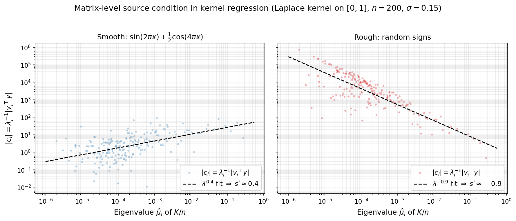
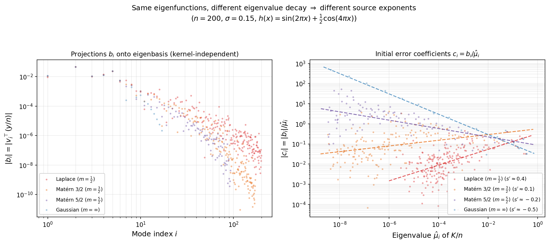
Numerical illustration. The figures below demonstrate this on a Laplace kernel ($\sigma = 0.15$) with $n = 200$ points drawn uniformly from $[0,1]$. The first figure plots the initial-error coefficients $\lvert c_i\rvert$ versus $\hat\mu_i$ on a log-log scale; the slope of the log-log fit directly reveals the matrix-level source parameter $s’$ that enters Theorem 7.1. For a smooth target $h(x) = \sin(2\pi x) + \tfrac12\cos(4\pi x)$ (left panel), the fitted slope is $s’ \approx 0.4$, so Theorem 7.1 predicts rate $O(k^{-1.8})$. For a rough target of random signs (right panel), the fitted slope is $s’ \approx -0.9$: the initial error is concentrated in the small-eigenvalue directions, so no source condition holds.
The next figure explains why the source exponent changes across kernels. For translation-invariant kernels on $[0,1]$, the eigenfunctions are approximately the same (Fourier modes), so the projections $b_i = v_i^\top(y/n)$ are nearly kernel-independent (left panel: all four kernels overlap). What differs is the eigenvalue decay: $\lambda_i \asymp i^{-\alpha}$ with $\alpha = 2$ (Laplace), $4$ (Matérn 3/2), $6$ (Matérn 5/2), or super-polynomial (Gaussian). Since $c_i = b_i/\lambda_i$, dividing by faster-decaying eigenvalues inflates the high-index coefficients more, producing a less favorable slope (right panel). If $b_i \propto i^{-r}$ for some target-dependent $r$, then $c_i \propto \lambda_i^{r/\alpha - 1}$, giving $s’ = r/\alpha - 1$. As $\alpha$ increases, $s’$ decreases — not because the target projects differently, but because each eigenvalue is smaller and dividing by it inflates $c_i$ more.
We now show how the source condition controls the rate of convergence of gradient descent. The GD rate is $O(k^{-(1+2s)})$, with two distinct payoffs depending on the sign of $s$:
-
(faster rate when $s > 0$). The rate $O(\lVert w\rVert^2\cdot k^{-(1+2s)})$ is strictly faster than $O(\lVert e_0\rVert^2\cdot k^{-1})$. The source condition concentrates the initial error on large-eigenvalue directions, which GD resolves quickly.
-
(dimension-free rate when $s \in (-\tfrac{1}{2}, 0)$). The rate $O(\lVert w\rVert^2/ k^{1+2s})$ is slower than $O(\lVert e_0\rVert^2/k)$ in terms of $k$, but the bound depends on $\lVert w\rVert^2$ rather than $\lVert e_0\rVert^2$. For polynomial eigenvalue decay $\lambda_i \asymp i^{-\alpha}$ with isotropic $w$, the initial error scales as
Therefore, the vanilla bound diverges as $n \to \infty$, whereas the source-condition bound $O(\lVert w\rVert^2/ k^{1+2s})$ is independent of $n$.
Theorem 7.1 (GD with source condition). If the initial error satisfies $e_0 = A^s w$ for some $s > -\tfrac{1}{2}$, then GD with $\eta = 1/\beta$ satisfies
\[f(x_k) - f^\ast \leq \frac{\beta^{1+2s}}{2}\left(\frac{1+2s}{2k+1+2s}\right)^{1+2s}\|w\|^2. \tag{13}\]In particular, $f(x_k) - f^\ast = O\left(\beta^{1+2s}\,k^{-(1+2s)}\,\lVert w\rVert ^2\right)$ as $k \to \infty$.
Proof. For GD with stepsize $\eta = 1/\beta$, the error satisfies $e_k = (I - A/\beta)^k e_0$, so
\[f(x_k) - f^\ast = \frac{1}{2}\sum_{i=1}^d \lambda_i\,(1-\lambda_i/\beta)^{2k}\,c_i^2.\]Writing $c_i = \lambda_i^s \tilde{c}_i$ with $\tilde{c}_i = v_i^\top w$, this becomes
\[f(x_k) - f^\ast = \frac{1}{2}\sum_{i=1}^d \lambda_i^{1+2s}\,(1-\lambda_i/\beta)^{2k}\,\tilde{c}_i^2,\]and therefore
\[f(x_k) - f^\ast \leq \frac{\|w\|^2}{2}\,\max_{\lambda \in [0,\beta]}\, \lambda^{1+2s}(1-\lambda/\beta)^{2k}. \tag{14}\]It suffices to maximize $g(t) = t^{1+2s}(1-t)^{2k}$ over $t \in [0,1]$, with the identification $\lambda = \beta t$. An elementary computation shows
\[\max_{t\in [0,1]}g(t) = \left(\frac{1+2s}{2k+1+2s}\right)^{1+2s}\left(\frac{2k}{2k+1+2s}\right)^{2k} \leq \left(\frac{1+2s}{2k+1+2s}\right)^{1+2s}.\]Multiplying by $\beta^{1+2s}/2$ and $\lVert w\rVert ^2$ gives the bound $(13)$. $\square$
The source condition can also be exploited by time-varying stepsizes. The relevant polynomial problem is now
\[\min_{\substack{p \in \mathcal P_k^r\\ p(0)=1}} \max_{\lambda \in [0,\beta]} \lambda^{1+2s}p(\lambda)^2.\]After the affine change of variables $\lambda = \frac{\beta}{2}(1-t)$, this becomes a minimax problem on $[-1,1]$ with weight $(1-t)^{1+2s}$. The solutions of this extremal problem are the Jacobi polynomials. You will derive this minimax construction in the next homework and will prove the following theorem.
Theorem 7.2 (Time-varying stepsizes with source condition). For every $s > -\tfrac{1}{2}$ and every horizon $k \geq 1$, there exists a sequence of stepsizes $\eta_1,\dots,\eta_k$ such that the corresponding GD iterate satisfies
\[f(x_k)-f^\ast \leq C_s\,\beta^{1+2s}\,k^{-2(1+2s)}\,\|w\|^2. \tag{15}\]where $C_s>0$ depends only on $s$.
In particular, the rate goes from $O(k^{-2})$ for Chebyshev accelerated GD without the source condition to $O(k^{-2(1+2s)})$ when the source condition holds. In principle, the stepsizes in the theorem are given by the reciprocals of the roots of the relevant Jacobi polynomial, and depend explicitly on $s$. This is not a serious drawback, however, because the same convergence rate is inherited by the conjugate gradient method, which achieves it adaptively without needing the stepsizes explicitly.
Corollary 7.1 (CG with source condition). If the initial error satisfies $e_0 = A^s w$ for some $s > -\tfrac{1}{2}$, then the CG iterates satisfy
\[f(x_k^{\mathrm{CG}})-f^\ast \leq C_s\,\beta^{1+2s}\,k^{-2(1+2s)}\,\|w\|^2,\]and CG terminates in at most $m$ iterations, where $m$ is the number of distinct nonzero eigenvalues of $A$.
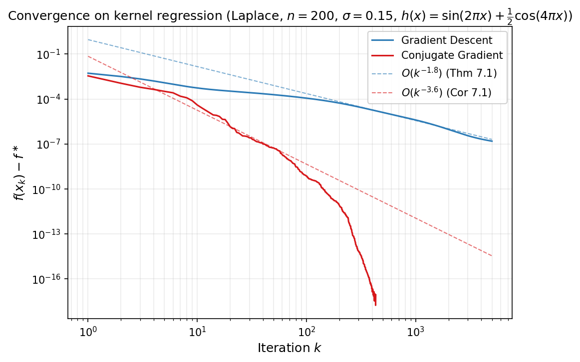
The following figure shows the actual convergence of gradient descent (with stepsize $\eta = 1/\beta$) and conjugate gradient on the smooth target for kernel regression. The dashed lines show the predicted rates: $O(k^{-1.8})$ for GD (Theorem 7.1) and $O(k^{-3.6})$ for CG (Corollary 7.1). Both methods track their predicted rates well.
The spectral integral
Source conditions improve rates by considering structure in the initial error. A complementary improvement comes from considering structure in the eigenvalue distribution. Recall from $(12)$ that for any first-order method whose error has the form $e_k = p_k(A)\,e_0$ for some polynomial $p_k \in \mathcal{P}_k$ with $p_k(0)=1$ — which includes gradient descent with stepsizes $\eta_j$ (where $p_k(\lambda) = \prod_j(1-\eta_j\lambda)$), the Chebyshev iteration, and the conjugate gradient method (which adaptively minimizes over $p_k$) — we have
\[f(x_k) - f^\ast = \frac{1}{2}\sum_{i=1}^d \lambda_i\,p_k(\lambda_i)^{2}\,c_i^2,\]where $c_i$ are the coordinates of $e_0$ in the eigenbasis of $A$. The idea is that if $d$ is large and the eigenvalues are well-spread out, the sum in the expression may be estimated as an integral with respect to a continuous density. To make this precise define the spectral error measure
\[\mu = \sum_{i=1}^d c_i^2\,\delta_{\lambda_i},\]where $\delta_{\lambda_i}$ is a Dirac delta measure. Observe that $\mu([0,\beta]) = \lVert e_0\rVert ^2$ and the error can be written as an integral:
\[f(x_k) - f^\ast = \frac{1}{2}\int_0^\beta \lambda\,p_k(\lambda)^{2}\,d\mu(\lambda). \tag{16}\]When $d$ is large and the eigenvalues are well-spread, the discrete measure $\mu$ is well-approximated by a continuous density. Suppose $d\mu(\lambda) \approx \phi(\lambda)\,d\lambda$ for a nonnegative function $\phi$—the spectral error density. The density $\phi$ encodes both the eigenvalue distribution and the initial error profile: if the eigenvalue density of $A$ is $\rho_A$ and the error components are roughly uniform ($c_i^2 \approx \lVert e_0\rVert ^2/d$), then $\phi(\lambda) \approx \lVert e_0\rVert ^2\rho_A(\lambda)$. Note that $\phi$ need not be integrable; what matters is that the error integral $(16)$, which has an extra factor of $\lambda$, converges.
Under this approximation, $f(x_k) - f^\ast \approx \mathcal{E}_k$, where
\[\mathcal{E}_k := \frac{1}{2}\int_0^\beta \lambda\,p_k(\lambda)^{2}\,\phi(\lambda)\,d\lambda.\]In particular, for fixed-stepsize GD with $\eta = 1/\beta$, we have $p_k(\lambda) = (1-\lambda/\beta)^k$ and the integrand $\lambda(1-\lambda/\beta)^{2k}$ is sharply peaked near its maximizer $\lambda^\ast = \beta/(2k+1)$ for large $k$, decaying rapidly away from this point. The animation below illustrates this concentration: as $k$ grows the peak narrows and shifts toward zero.
The integral is therefore controlled by the behavior of $\phi$ near $\lambda^\ast$—which shifts toward zero as $k$ grows. The next two subsections exploit this concentration to obtain convergence rates that depend on the spectral density.
Power-law spectral density
When the spectral error density follows a power law near the origin:
\[\phi(\lambda) = M\,\lambda^{a-1} \qquad \text{on } (0, \beta],\]the exponent $a$ controls the spectral mass near zero. For $a > 1$, the density vanishes at zero (few eigenvalues near the origin); for $a = 1$, the density is flat; for $0 < a < 1$, the density diverges but remains integrable.
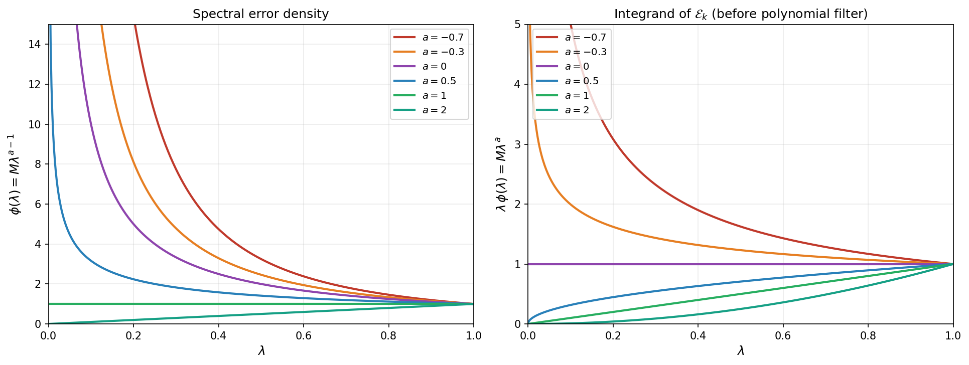
The figure below illustrates the three regimes. The left panel plots the spectral error density $\phi(\lambda) = M\lambda^{a-1}$: for $a > 1$ it vanishes at the origin, for $a = 1$ it is flat, and for $a < 1$ it diverges (still integrable when $a > 0$). The right panel plots the integrand $\lambda\,\phi(\lambda) = M\lambda^a$ that appears in the spectral integral $\mathcal{E}_k$: even when $\phi$ itself is non-integrable ($a \leq 0$), the extra $\lambda$ factor makes the integrand integrable whenever $a > -1$.
Example (polynomial eigenvalue decay). Kernels such as Laplace and Matérn have eigenvalues that decay polynomially: $\lambda_i \asymp i^{-\alpha}$ for some $\alpha > 0$. To find the corresponding spectral exponent $a$, we can compute the eigenvalue density $\rho_A$. The empirical CDF of the eigenvalues is $F(\lambda) = \tfrac{1}{d}\cdot \lvert\lbrace i:\lambda_i \leq \lambda\rbrace \rvert$. Since $\lambda_i = Ci^{-\alpha}$ is decreasing, $\lambda_i \leq \lambda$ iff $i \geq (C/\lambda)^{1/\alpha}$, so
\[F(\lambda) \approx 1 - \frac{(C/\lambda)^{1/\alpha}}{d} = 1 - \frac{C^{1/\alpha}}{d}\,\lambda^{-1/\alpha}.\]Differentiating gives $\rho_A(\lambda) = F’(\lambda) \propto \lambda^{-1/\alpha - 1}$. With isotropic error ($c_i^2 \approx \lVert e_0\rVert^2/d$), the spectral error density is $\phi(\lambda) \propto \lambda^{-1/\alpha - 1}$. Matching to $\phi = M\lambda^{a-1}$ gives $a = -1/\alpha$.
Since $a = -1/\alpha < 0$, the total mass $\lVert e_0\rVert^2 = \int \phi\,d\lambda$ diverges—the density $\phi(\lambda) \propto \lambda^{-1/\alpha-1}$ has a non-integrable singularity at $\lambda = 0$. In kernel regression (starting from $x_0 = 0$), this has a concrete interpretation: the initial error is $e_0 = A^{-1}b$, so its spectral coefficients are $c_i = b_i/\lambda_i$. Because $\lambda_i \to 0$ polynomially, the coefficients $c_i$ grow for modes with small eigenvalues. As $n$ increases, more and more modes with tiny eigenvalues appear, each contributing a large $c_i^2$ term, and $\lVert e_0\rVert^2 = \sum c_i^2$ diverges. In particular, the vanilla rate $O(\lVert e_0\rVert ^2/k)$ becomes meaningless.
Suppose more generally that $c_i$ satisfy a source condition $e_0 = A^s w$, and therefore $c_i = \lambda_i^s w_i$. If in addition, the coordinates $w_i$ are isotropic ($w_i^2 \approx \lVert w\rVert^2/d$), the spectral error density becomes $\phi(\lambda) \propto \lambda^{2s}\rho_A(\lambda) \propto \lambda^{- \tfrac{1}{\alpha} - 1+2s}$. The source condition counteracts the $1/\lambda_i$ blow-up: $c_i = \lambda_i^s w_i$ decays with the eigenvalues.
We are now ready to derive the rate of convergence of gradient descent under the power-law spectrum.
Theorem 7.2 (Power-law spectral density). Assume the spectral error density is $\phi(\lambda)=M\lambda^{a-1}$ on $(0,\beta]$ for some $M>0$ and $a>-1$. Then the GD iterates with $\eta = 1/\beta$ satisfy
\[\mathcal{E}_k = \frac{M\,\beta^{a+1}}{2}\cdot\frac{\Gamma(a+1)\,\Gamma(2k+1)}{\Gamma(2k+a+2)}.\]In particular, as $k \to \infty$, we have
\[\mathcal{E}_k \sim \frac{M\,\Gamma(a+1)\,\beta^{a+1}}{2\,(2k)^{a+1}}. \tag{17}\]Proof. Substituting $t = \lambda/\beta$ yields
\[\int_0^\beta \lambda^{a}(1-\lambda/\beta)^{2k}\,d\lambda = \beta^{a+1}\int_0^1 t^{a}(1-t)^{2k}\,dt = \beta^{a+1}\,B(a+1,\, 2k+1),\]where $B(p,q) = \Gamma(p)\Gamma(q)/\Gamma(p+q)$ is the Beta function. The asymptotics follow from the standard estimate $\Gamma(n+c)/\Gamma(n) \sim n^c$ as $n \to \infty$, applied with $n = 2k+1$ and $c = a+1$. $\square$
Relationship to the $O(1/k)$ bound. The vanilla $O(1/k)$ bound of Theorem 6.1 is a max-bound: it replaces the spectral filter $\lambda(1-\lambda/\beta)^{2k}$ by its pointwise maximum over $\lambda$, then pulls the maximum outside the integral:
\[\mathcal{E}_k \leq \frac{1}{2}\max_{\lambda}\bigl[\lambda(1-\lambda/\beta)^{2k}\bigr]\int_0^\beta \phi(\lambda)\,d\lambda \leq \frac{\beta}{2(2k+1)}\lVert e_0\rVert^2.\]The price is that the entire initial error norm $\lVert e_0\rVert^2 = \int \phi\,d\lambda$ appears as a single constant, discarding all information about where in the spectrum the error lives. The spectral integral keeps $\phi(\lambda)$ inside the integral, so the rate reflects the spectral distribution of the error, not just its total size. Concretely, two things can happen:
-
$\lVert e_0\rVert^2$ is finite but the error concentrates on large eigenvalues ($a > 0$). The spectral integral gives $O(k^{-(a+1)})$ with $a+1 > 1$, strictly faster than $O(1/k)$. The vanilla bound is finite but wasteful because it treats all eigenvalue directions equally.
-
$\lVert e_0\rVert^2 \approx \infty$ ($-1 < a \leq 0$, e.g. polynomial eigenvalue decay without a source condition). The vanilla bound gives $\infty$—it says nothing. But the spectral integral is still finite because the $\lambda$ factor in the integrand $\lambda(1-\lambda/\beta)^{2k}\phi(\lambda) = M\lambda^a(1-\lambda/\beta)^{2k}$ vanishes at $\lambda = 0$, canceling the singularity of $\phi$. The result is a finite bound $O(k^{-(a+1)})$ with $0 < a+1 \leq 1$.
The following table summarizes these regimes in general.
| Exponent $a$ | $\lVert e_0\rVert^2 = \int\phi$ | Rate | vs.\ $O(1/k)$ bound |
|---|---|---|---|
| $a \geq 0$ | finite ($a>0$) or $\infty$ ($a=0$) | $O(k^{-(a+1)})$, $a+1\geq 1$ | improves on $O(1/k)$ |
| $-1 < a < 0$ | $\infty$ | $O(k^{-(a+1)})$, $a+1<1$ | $O(1/k)$ bound is vacuous; spectral integral is the only finite bound |
Example (Matérn kernels in $\mathbb{R}^p$). A Matérn-$m$ kernel in dimension $p$ has eigenvalue decay $\lambda_i \asymp i^{-(2m+p)/p}$, so $\alpha = (2m+p)/p$ and the base spectral exponent is $a = -p/(2m+p)$. A source condition $e_0 = A^s w$ with isotropic $w$ shifts this to $a_{\mathrm{eff}} = 2s - \tfrac{p}{2m+p}$, giving the rate $\mathcal{E}_k = O(k^{-(2s + 1 - \frac{p}{2m+p})})$. The table below lists several concrete cases in $p=1$.
| Kernel | $m$ | $a$ (no source) | Rate ($s=0$) | $a_{\mathrm{eff}}$ ($s=\tfrac{1}{2}$) | Rate ($s=\tfrac{1}{2}$) |
|---|---|---|---|---|---|
| Laplace | $\tfrac{1}{2}$ | $-\tfrac{1}{2}$ | $O(k^{-1/2})$ | $\tfrac{1}{2}$ | $O(k^{-3/2})$ |
| Matérn 3/2 | $\tfrac{3}{2}$ | $-\tfrac{1}{4}$ | $O(k^{-3/4})$ | $\tfrac{3}{4}$ | $O(k^{-7/4})$ |
| Matérn 5/2 | $\tfrac{5}{2}$ | $-\tfrac{1}{6}$ | $O(k^{-5/6})$ | $\tfrac{5}{6}$ | $O(k^{-11/6})$ |
Without a source condition ($s=0$), the rate is always slower than $O(1/k)$ and the vanilla bound is vacuous ($\lVert e_0\rVert^2 = \infty$). With even a modest source condition $s = \tfrac{1}{2}$, the effective exponent flips to $a_{\mathrm{eff}} > 0$ and the rate becomes faster than $O(1/k)$. Smoother kernels (larger $m$) are closer to the $O(1/k)$ threshold in both directions: the penalty without a source condition is milder, but so is the improvement with one. Increasing $p$ makes everything harder: the base exponent $a = -p/(2m+p)$ is more negative, so a stronger source condition is needed to cross the $O(1/k)$ boundary ($s > p/(2(2m+p))$).
Crucially, the spectral integral bound depends on the density parameter $M$, not on the total mass $\lVert e_0\rVert^2 = \int \phi\,d\lambda$. For Matérn kernels with $a < 0$, the norm $\lVert e_0\rVert^2$ diverges as $n \to \infty$, making the vanilla $O(1/k)$ constant blow up. The spectral integral remains finite because the filter $\lambda(1-\lambda/\beta)^{2k}$ automatically suppresses the small-eigenvalue directions responsible for the divergence. The result is a dimension-free rate: $M$ depends on the spectral shape, not the problem size.
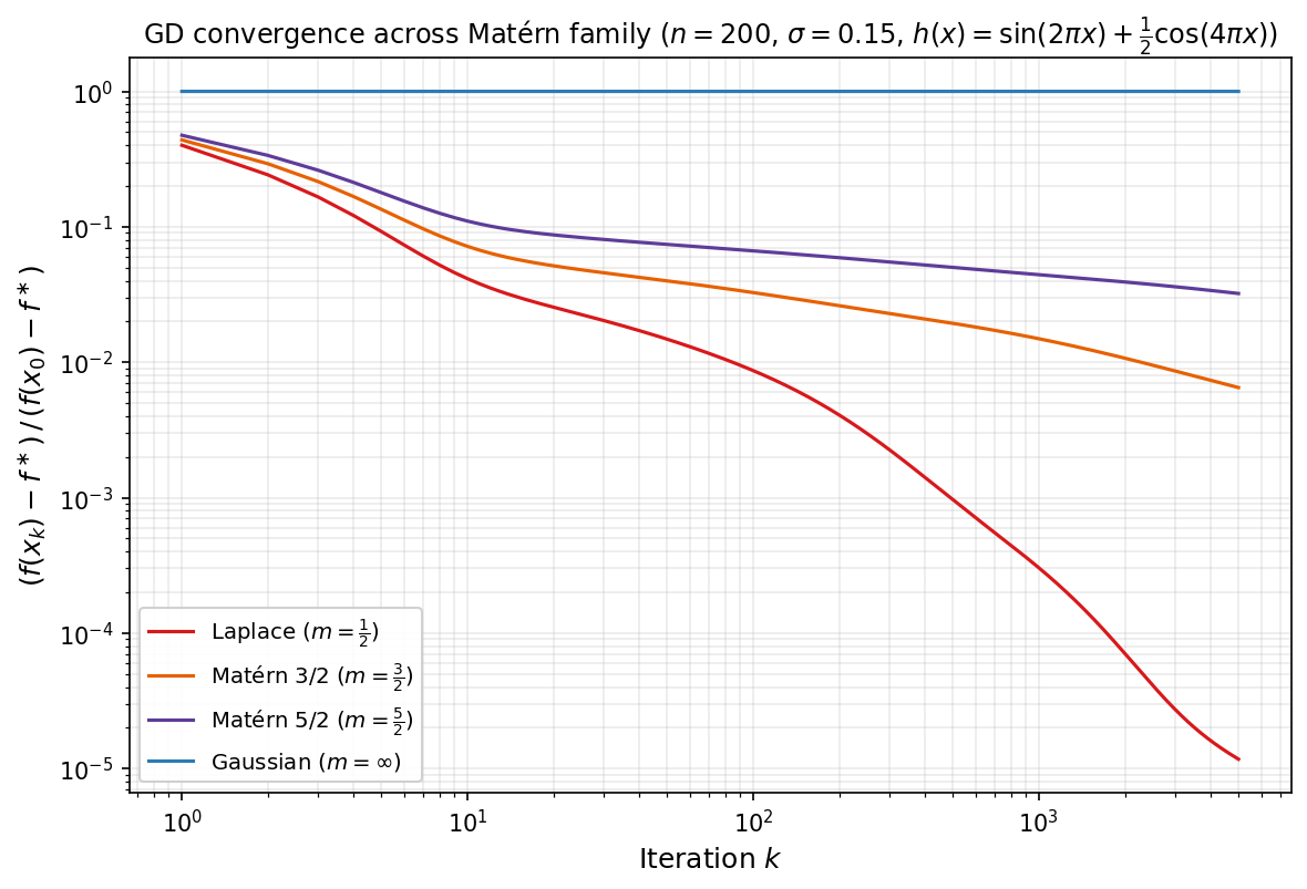
Effect of kernel smoothness. The figure below compares GD convergence on the same target function $h(x) = \sin(2\pi x) + \tfrac{1}{2}\cos(4\pi x)$ across the Matérn family: Laplace ($m=\tfrac12$), Matérn 3/2, Matérn 5/2, and Gaussian. The y-axis shows the relative gap $(f(x_k)-f^\ast)/(f(x_0)-f^\ast)$. The ordering is striking and at first glance counter-intuitive: rougher kernels converge faster. The Gaussian kernel makes essentially no progress in 5000 iterations, while the Laplace kernel reduces the gap by five orders of magnitude.
The initial error norms illustrate the divergence phenomenon discussed above. With $n=200$ points and the same target, the initial function gaps $f(x_0)-f^\ast$ are nearly identical across the first three kernels ($\approx 0.01$), yet $\lVert e_0\rVert^2$ explodes as the kernel gets smoother:
| Kernel | $\lVert e_0\rVert^2$ | $f(x_0)-f^\ast$ | $\kappa$ |
|---|---|---|---|
| Laplace | $\approx 1$ | $\approx 0.013$ | $1.4 \times 10^5$ |
| Matérn 3/2 | $\approx 700$ | $\approx 0.012$ | $1.1 \times 10^{10}$ |
| Matérn 5/2 | $\approx 3\times 10^8$ | $\approx 0.012$ | $1.8 \times 10^{14}$ |
| Gaussian | $\approx 5\times 10^{39}$ | $\approx 2.5 \times 10^{9}$ | $3.6 \times 10^{29}$ |
The function gap (which contains the stabilizing $\lambda_i$ factor) is dimension-stable, but $\lVert e_0\rVert^2$ grows by 40 orders of magnitude from Laplace to Gaussian. This is exactly why the vanilla $O(1/k)$ bound — which uses $\lVert e_0\rVert^2$ as its constant — becomes meaningless for smooth kernels, while the spectral integral remains informative.
The Laplace method for positive definite spectra
When $A \succ 0$, the eigenvalues lie in $[\alpha, \beta]$ with $\alpha > 0$, and the base rate of convergence for GD is exponential: $O((1-\alpha/\beta)^{2k})$. The spectral integral can still yield improvements, but they take the form of a polynomial correction to the exponential rate rather than a change in the polynomial exponent. The argument is based on the so-called Laplace estimate for integrals of exponential functions.
Theorem 7.3 (Laplace upper bound). Let $A \succ 0$ with eigenvalues in $[\alpha, \beta]$, and suppose the spectral error density $\phi$ satisfies
\[\phi(\lambda) \leq C\,(\lambda - \alpha)^p \qquad \textit{on } [\alpha, \beta]\]for constants $C > 0$ and $p > -1$. Then for every $k \geq 1$ the GD iterates with $\eta = 1/\beta$ satisfy
\[\mathcal{E}_k \leq \frac{C\,\Gamma(p+1)}{2}\left[\alpha + \frac{(p+1)(\beta-\alpha)}{2k}\right]{\left(\frac{\beta-\alpha}{2k}\right)^{p+1}\left(1-\kappa^{-1}\right)^{2k}}. \tag{18}\]In particular, the leading term is $\tfrac{C\,\alpha\,\Gamma(p+1)}{2}\bigl(\tfrac{\beta-\alpha}{2k}\bigr)^{p+1}(1-\kappa^{-1})^{2k}$, and the bracketed correction is $1 + O(1/k)$.
Proof. Substitute $u = \lambda - \alpha$ in $\mathcal{E}_k$ to get
\[\mathcal{E}_k = \frac{1}{2}\int_0^{\beta-\alpha} (\alpha + u)\,\bigl(1 - \tfrac{\alpha+u}{\beta}\bigr)^{2k}\,\phi(\alpha + u)\,du.\]Next, factor out the dominant exponential using the identity
\[1-\tfrac{\alpha+u}{\beta} = (1-\tfrac{\alpha}{\beta})(1 - \tfrac{u}{\beta - \alpha})\]to get
\[\mathcal{E}_k= \frac{(1-\kappa^{-1})^{2k}}{2}\int_0^{\beta-\alpha} (\alpha + u)\left(1 - \frac{u}{\beta-\alpha}\right)^{2k}\phi(\alpha + u)\,du.\]Using the hypothesis $\phi(\alpha+u)\leq Cu^p$, we bound the last integral by
\[C\int_0^{\beta-\alpha}\bigl[\alpha\,u^p + u^{p+1}\bigr]\left(1-\tfrac{u}{\beta-\alpha}\right)^{2k}du.\]For each exponent $q \in \lbrace p, p+1\rbrace$, the substitution $v = 2ku/(\beta-\alpha)$ gives
\[\int_0^{\beta-\alpha} u^q\left(1-\tfrac{u}{\beta-\alpha}\right)^{2k}du \;=\; \left(\tfrac{\beta-\alpha}{2k}\right)^{q+1}\!\!\int_0^{2k} v^q\left(1-\tfrac{v}{2k}\right)^{2k}dv \;\leq\; \left(\tfrac{\beta-\alpha}{2k}\right)^{q+1}\Gamma(q+1),\]where in the last step we used the pointwise inequality $(1-v/(2k))^{2k}\leq e^{-v}$ on $[0,2k]$ and extended the integral to $[0,\infty)$. Combining the two cases ($q = p, p+1$) and using equality $\Gamma(p+2) = (p+1)\Gamma(p+1)$, we deduce
\[\mathcal{E}_k \;\leq\; \frac{C\,(1-\kappa^{-1})^{2k}}{2}\left(\frac{\beta-\alpha}{2k}\right)^{p+1}\Gamma(p+1)\left[\alpha + \frac{(p+1)(\beta-\alpha)}{2k}\right],\]which completes the proof. $\square$
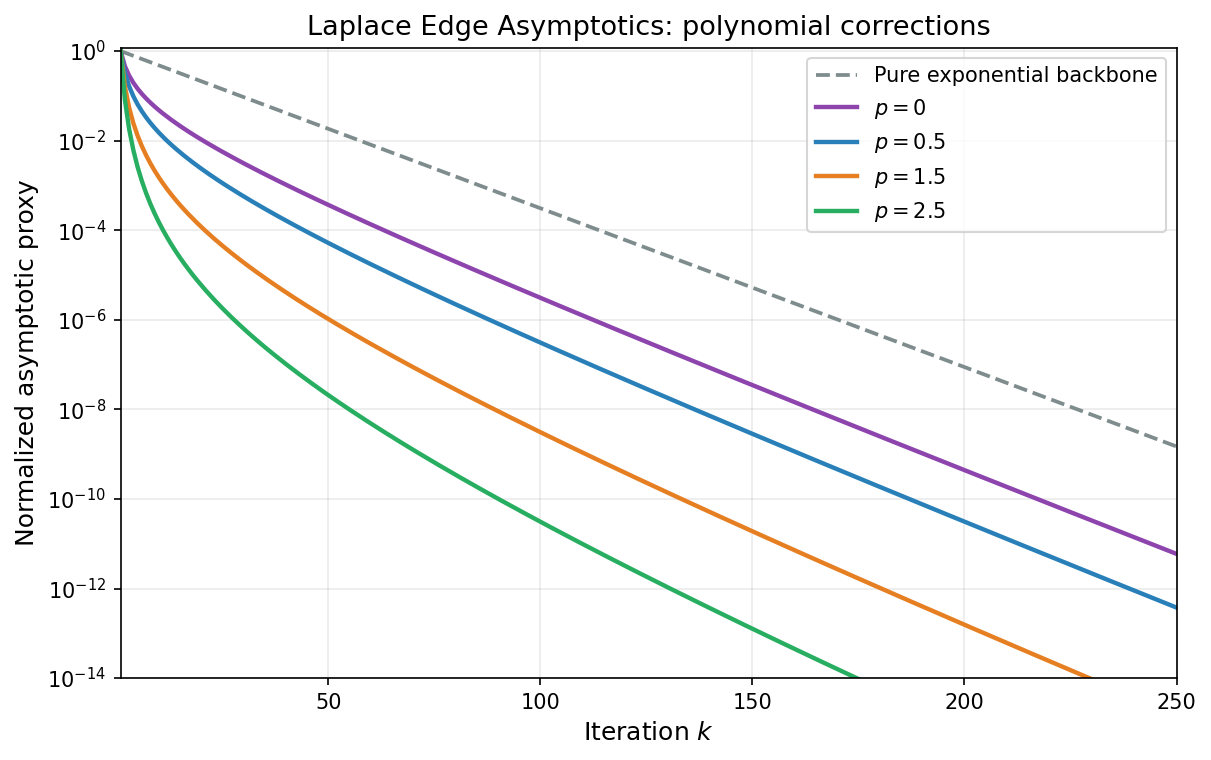
Compared with the worst-case bound $f(x_k) - f^\ast \leq (1-\alpha/\beta)^{2k}(f(x_0)-f^\ast)$, the Laplace estimate reveals a polynomial improvement of order $k^{-(p+1)}$ that depends on how the spectral density vanishes at the left edge of the spectrum. A flat density ($p = 0$) gives a $1/k$ improvement; a square-root vanishing ($p = 1/2$) gives $k^{-3/2}$; higher-order vanishing gives even larger gains.
The figure below compares several edge exponents $p$ against the same exponential backbone, showing the progressive polynomial correction predicted by Theorem 7.3.
Application: Marchenko–Pastur spectrum
We now specialize to the linear least-squares setting from the beginning of the notes, but with a random design matrix $D\in\mathbb{R}^{n\times d}$ whose entries are iid with zero mean and unit variance. Consider
\[\min_{x\in\mathbb{R}^d} \frac{1}{2n}\|Dx-y\|^2.\]This is exactly the quadratic problem from Section 1, equivalently the problem of solving the normal equations $Ax=b$, with
\[A=\frac{1}{n}D^\top D,\qquad b=\frac{1}{n}D^\top y.\]The Marchenko–Pastur distribution arises as the limiting spectral distribution of the sample covariance / Gram matrix $A = \tfrac{1}{n}D^\top D$ when the entries of $D \in \mathbb{R}^{n \times d}$ are iid with zero mean and unit variance, in the proportional asymptotic regime
\[\tfrac{d}{n} \to \gamma > 0\qquad \textrm{as}\qquad n\to \infty.\]Here, convergence is meant in the following precise sense. Letting $\lambda_1(A),\dots,\lambda_d(A)$ denote the eigenvalues of $A$, define the empirical spectral measure
\[\hat{\mu}_A \;=\; \frac{1}{d}\sum_{i=1}^{d}\delta_{\lambda_i(A)},\]Note that this measure is itself random because $A$ is random. Marchenko and Pastur showed that $\hat{\mu}_A$ weakly converges to a deterministic limit measure $\mu_{\mathrm{MP}}$, called Marchenko–Pastur law. That is for any bounded continuous function $f$, it holds:
\[\int f\,d\hat{\mu}_A \;\xrightarrow[n\to\infty]{\text{a.s.}}\; \int f\,d\mu_{\mathrm{MP}}.\]This type of weak convergence is denoted $\hat{\mu}_A\;\Rightarrow\;\mu_{\mathrm{MP}}$.
The animation below illustrates this convergence for the three regimes $\gamma \in \lbrace 0.5,\,1,\,2\rbrace $ (with iid standard Gaussian entries in $D$). For each frame a fresh $D$ is drawn at the given $n$, the $d$ eigenvalues of $A=\tfrac{1}{n}D^\top D$ are computed, and their empirical frequency density is plotted: the eigenvalues are sorted into equal-width bins $\lbrace B_j\rbrace $ on the $\lambda$-axis, and each bin height equals
\[\frac{\#\{i:\lambda_i(A) \in B_j\}}{d \cdot \lvert B_j\rvert},\]so that the total area of the histogram equals $1$ (matching the mass of $\hat{\mu}_A$). As $n$ grows, this histogram collapses onto the Marchenko–Pastur density curve overlaid in black. In the rank-deficient case $\gamma = 2$ the matrix $A$ has exactly $d - n$ zero eigenvalues, which form an atom of mass $1-1/\gamma$ at $\lambda=0$ in $\hat\mu_A$; those are excluded from the histogram, so the bulk integrates to the remaining mass $1/\gamma$ and aligns with $\rho_{\mathrm{MP}}$ on $[\lambda_-,\lambda_+]$.
Concretely, $\mu_{MP}$ admits the decomposition
\[\mu_{MP} \;=\; \max\!\left(0,\;1-\tfrac{1}{\gamma}\right)\,\delta_{0} \;+\; \rho_{MP}(\lambda)\,d\lambda,\]consisting of (i) a point mass at $\lambda=0$ of weight $\max(0,\,1-1/\gamma)$, which is nonzero only when $\gamma > 1$ and accounts for the $d-n$ forced zero eigenvalues of $A$, and (ii) an absolutely continuous part supported on $[\lambda_-,\lambda_+]$ with density
\[\rho_{MP}(\lambda) = \frac{\sqrt{(\lambda_+ - \lambda)(\lambda - \lambda_-)}}{2\pi\gamma\,\lambda}, \qquad \lambda \in [\lambda_-, \lambda_+],\]where $\lambda_\pm := (1 \pm \sqrt{\gamma})^2$. The continuous part carries total mass $\min(1,\,1/\gamma)$, so together with the atom the measure integrates to $1$.
To connect the Marchenko–Pastur law with the spectral integral bounds, we assume directly that the reweighted empirical spectral measure
\[\nu_d:=\sum_{i=1}^d c_i^2\,\delta_{\lambda_i}\]has the same asymptotic shape as the empirical spectral measure of $A$, that is
\[\nu_d \;\Rightarrow\; \lVert e_0\rVert^2\,\mu_{MP}, \qquad \text{a.s. as } n\to\infty,\ d/n\to\gamma.\]This is the only property used below and holds for example if we initialize at $x_0=0$ and $x^{\ast}\sim \mathcal{N}(0,\frac{R}{d}I_d)$ for any constant $R>0$.
Let us now look at the convergence of GD for the least squares problem.
- $\gamma < 1$ (no atom at zero). Here $\lambda_- > 0$ and therefore $n>d$. This setting is relevant for linear regression with more feature vectors $(n)$ than the dimension of the space $(d)$. The problem is positive definite with
Near the left edge $\lambda_-$, the density vanishes like a square root:
\[\rho_{MP}(\lambda) \sim \frac{\sqrt{(\lambda_+ - \lambda_-)(\lambda - \lambda_-)}}{2\pi\gamma\,\lambda_-} = \frac{2\gamma^{1/4}\sqrt{\lambda - \lambda_-}}{2\pi\gamma\,(1-\sqrt\gamma)^2} \quad \text{as } \lambda \to \lambda_-^+.\]With isotropic initialization, Theorem 7.3 applies with $\alpha = \lambda_-$, $\beta = \lambda_+$, and $p = 1/2$. Since $\Gamma(3/2) = \sqrt\pi/2$, the estimate $(18)$ gives
\[\mathcal{E}_k \sim \frac{\tilde{C}(\gamma)}{k^{3/2}}\left(1 - \frac{1}{\kappa}\right)^{2k}\|e_0\|^2 \quad \text{as } k \to \infty,\]where $\tilde{C}(\gamma)$ is an explicit constant depending on the aspect ratio $\gamma$.
- $\gamma = 1$ (hard edge at zero). This is the case of a square data matrix $n=d$. Then the left edge is $\lambda_-=0$ and
Thus under isotropic initialization $\phi(\lambda) \sim \tfrac{\lVert e_0\rVert^2}{\pi}\,\lambda^{-1/2}$ near $\lambda=0$ (power-law exponent $a=1/2$ in Theorem 7.2 with $s=0$, $M = \lVert e_0\rVert^2/\pi$, $\beta = 4$). The asymptotic $(17)$ then gives
\[\mathcal{E}_k \;\sim\; \frac{\lVert e_0\rVert^2}{\sqrt{2\pi}\,k^{3/2}} \qquad \text{as } k \to \infty.\]- $\gamma > 1$ (rank deficient). The empirical spectrum has an atom at $0$ of asymptotic mass $1-1/\gamma$, so globally $\alpha=0$. However, the nonzero spectrum still lies in $[(\sqrt{\gamma}-1)^2,\ (\sqrt{\gamma}+1)^2]$. Since the objective gap carries the factor $\lambda$ in $(16)$, the nullspace part does not contribute to $f(x_k)-f^\ast$. Therefore the nonzero spectral component behaves as in the positive definite case, with
and the same asymptotic form
\[\mathcal{E}_k\sim \frac{\hat{C}(\gamma)}{k^{3/2}}\left(1-\frac{\alpha_{\mathrm{eff}}}{\beta}\right)^{2k}\|e_0\|^2.\]In all three regimes, the square-root edge behavior of Marchenko–Pastur yields the same $k^{-3/2}$ polynomial factor; what changes is whether it multiplies an exponential term (gap $>0$) or appears alone (gap $=0$).
Extensions to the Krylov method
We now turn to the analogous analysis for the Krylov method. Passing directly to the limit under the reweighted spectral assumption $\nu_d\Rightarrow\nu$ of the earlier subsections, finding the best stepsize sequence is equivalent to solving the polynomial problem
\[\mathcal{E}_k \;=\; \min_{\substack{p\in\mathcal{P}_k\\ p(0)=1}}\,\int_{0}^{\beta}\lambda\,p(\lambda)^2\,d\nu(\lambda), \tag{19}\]where $\nu$ is the limiting (reweighted) spectral measure supported on $[0,\beta]$ — for example $\nu=\lVert e_0\rVert^2\,\mu_{MP}$ in the Marchenko–Pastur setting — and $\mathcal{P}_k$ consists of degree at most $k$ polynomials. Note that the constraint set $\mathcal{V}_k:=\lbrace p\in \mathcal{P}_k: p(0)=1\rbrace$ is a finite-dimensional affine space.
Interestingly, we will now see that the solution to $(19)$ can be computed explicitly. The key idea is to realize that the objective has the form \(\lVert p\rVert^2\) where the norm is induced by the inner product \(\langle f,g\rangle=\int_{0}^{\beta} fg\,d\mu\) with reweighted measure \(d\mu(\lambda)=\lambda\cdot d\nu(\lambda)\). Let \(\psi_0,\dots,\psi_k\) be any orthonormal basis of \(\mathcal{P}_k\) with respect to this inner product; such a basis can be constructed analytically by Gram–Schmidt. Writing \(p=\sum_{i=0}^k u_i\,\psi_i\) for unknown coefficients \(u_i\), the optimization problem $(19)$ is equivalent to
\[\min_{u\in \mathbb{R}^{k+1}}\; \lVert u\rVert_2^2 \qquad \textrm{subject to}\qquad \sum_{i=0}^k u_i\psi_i(0)=1,\]which amounts to finding the minimum-norm vector in a hyperplane. The solution is the rescaled outward normal, with coordinates \(u_i=\psi_i(0)\big/\sum_{j=0}^k \psi_j(0)^2\). Therefore, the optimal polynomial $p$ that solves $(19)$ is
\[p^{\ast}(t)=\frac{\sum_{i=0}^{k}\psi_i(0)\psi_i(t)}{\sum_{i=0}^k \psi_i(0)^2}.\]Thus we have proved the following theorem.
Theorem 7.4 (Minimum-norm polynomial). Let $\psi_0,\dots,\psi_k$ be any orthonormal basis of $\mathcal{P}_k$ with respect to the inner product $\langle f,g\rangle=\int fg\,d\mu$, where $d\mu(\lambda)=\lambda\,d\nu(\lambda)$. Then the unique solution of $(19)$ is
\[p^\ast(t) \;=\; \frac{\sum_{i=0}^{k}\psi_i(0)\,\psi_i(t)}{\sum_{i=0}^{k}\psi_i(0)^2} \qquad \text{with minimal value}\quad \frac{1}{\sum_{i=0}^{k}\psi_i(0)^2}. \tag{20}\]We now apply Theorem 7.4 to the Marchenko–Pastur problem in the critical case $\gamma=1$. The orthogonal polynomials with respect to the corresponding measure turn out to be the Chebyshev polynomials of the second kind $U_k$.
Theorem 7.5 (CG on Marchenko–Pastur, critical case). Suppose $\gamma=1$ and the reweighted spectral assumption $\nu_d\Rightarrow \lVert e_0\rVert^2\,\mu_{MP}$ holds. Then for every $k\geq 1$, it holds:
\[\mathcal{E}_k \;=\; \frac{3\,\lVert e_0\rVert^2}{(k+1)(k+2)(2k+3)}. \tag{22}\]In particular, this is the rate achieved by the iterates of the CG algorithm.
Proof. Specializing the Marchenko–Pastur distribution to $\gamma=1$ yields
\[\rho_{MP}(\lambda) \;=\; \frac{\sqrt{4-\lambda}}{2\pi\sqrt{\lambda}}\qquad\textrm{on}\qquad[0,4].\]Therefore the measure $d\mu(\lambda):=\lambda\,\rho_{MP}(\lambda)\,d\lambda$ that appears in $(19)$ is
\[d\mu(\lambda) \;=\; \frac{\sqrt{\lambda(4-\lambda)}}{2\pi}\,d\lambda \qquad\textrm{on}\qquad [0,4],\]and minimizing the right-hand side of $(19)$ amounts to
\[\mathcal{E}_k \;=\; \frac{\lVert e_0\rVert^2}{2}\,\min_{\substack{p\in\mathcal{P}_k\\ p(0)=1}}\int_{0}^{4} p(\lambda)^2\,d\mu(\lambda).\]This is the abstract problem of Theorem 7.4. It suffices now to identify an orthogonal basis of $\mathcal{P}_k$ in $L^2(\mu)$. Apply the affine change of variables
\[x(\lambda) \;:=\; \frac{\lambda}{2}-1,\]which maps $[0,4]$ to $[-1,1]$. With this change of coordinates we have $\sqrt{\lambda(4-\lambda)}=2\sqrt{1-x^2}$ and $d\lambda=2\,dx$, hence $d\mu = \tfrac{2}{\pi}\sqrt{1-x^2}\,dx$. A standard fact is that the Chebyshev polynomials of the second kind $U_j$ from Section 6 are orthogonal on $[-1,1]$ with weight $\sqrt{1-x^2}$ and their square norm is $\int_{-1}^{1}U_j(x)^2\sqrt{1-x^2}\,dx=\pi/2$. Therefore
\[q_j(\lambda) \;:=\; U_j\!\bigl(x(\lambda)\bigr),\]is an orthonormal basis of $\mathcal{P}_k$ in $L^2(\mu)$. Using the identities $U_j(-1)=(-1)^j(j+1)$ and $U_j(1)=j+1$ from Section 6 gives $q_j(0)^2=(j+1)^2$. Substituting into the orthogonal-polynomial formula $(21)$ gives
\[\min_{\substack{p\in\mathcal{P}_k\\ p(0)=1}}\int_{0}^{4}p(\lambda)^2\,d\mu(\lambda) \;=\; \frac{1}{\sum_{j=0}^{k}(j+1)^2} \;=\; \frac{6}{(k+1)(k+2)(2k+3)},\]Multiplying by $\lVert e_0\rVert^2/2$ yields the bound $(22)$. $\square$
Two remarks comparing $(22)$ with the GD bound at $\gamma=1$ are in order.
-
Improvement over the universal CG bound. The universal CG bound from Theorem 6.3 gives $f(x_k^{\mathrm{CG}})-f^\ast=O(\lVert e_0\rVert^2/k^{2})$. The MP analysis improves this to $O(\lVert e_0\rVert^2/k^{3})$.
-
Comparison with GD. Contrasting $(22)$ with the GD asymptotic $\mathcal E_k\sim \lVert e_0\rVert^2/(\sqrt{2\pi}\,k^{3/2})$ derived in regime $2$ above, CG converges at the faster rate $k^{-3}$ at the critical aspect ratio.
Numerical illustration. The figure below confirms both rates on a random linear least-squares problem at the critical aspect ratio. We draw $D\in\mathbb R^{n\times n}$ with iid standard Gaussian entries ($n=d=1500$, so $\gamma=1$), form $A=\tfrac{1}{n}D^\top D$ (whose limiting spectrum is $\mu_{MP}$ on $[0,4]$), pick $x^\ast$ uniformly on the sphere of radius $\sqrt{n}$, and run GD with stepsize $\eta=1/\lambda_{\max}(A)$ and CG starting from $x_0=0$, plotting the median objective gap over $30$ independent trials (shaded bands show the $10$–$90\%$ interquantile range). Both curves match their predicted sublinear rates — $O(k^{-3/2})$ for GD and $O(k^{-3})$ for CG. The GD band is essentially invisible (the empirical rate is highly self-averaging across draws of $A$), while the CG band widens slightly in the tail, reflecting CG’s greater sensitivity to the random small-eigenvalue structure of $A$.
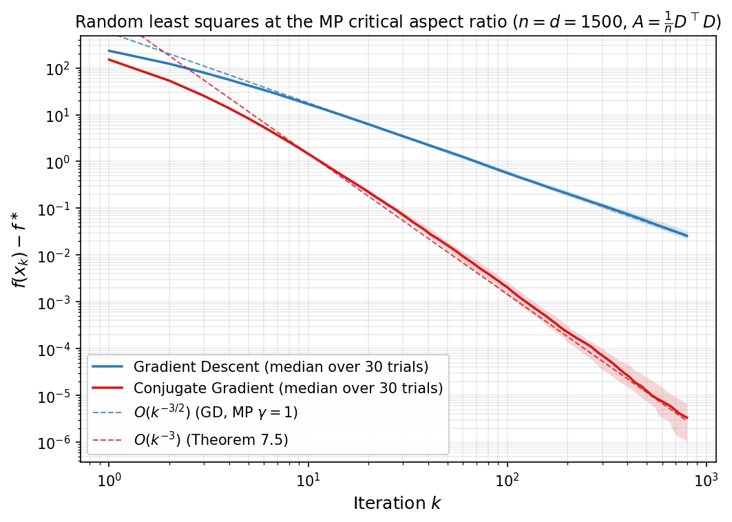
As the final application of the spectral integral approach, we now derive convergence of CG under a power-law spectrum. We assume the spectral error density is $\phi(\lambda)=M\lambda^{a-1}$ on $(0,\beta]$ for some $M>0$ and $a>-1$. The relevant measure is therefore $d\mu(\lambda):=\lambda\,\phi(\lambda)\,d\lambda=M\lambda^{a}\,d\lambda$. After the affine rescaling $x=2\lambda/\beta-1$ that maps $[0,\beta]$ to $[-1,1]$, this measure becomes $d\mu=M(\beta/2)^{a+1}(1+x)^{a}\,dx$, so the relevant orthogonal family is that of the classical Jacobi polynomials with parameters $(0,a)$. We briefly recall their definition and the three properties used in the proof below.
Jacobi polynomials. For parameters $p,q>-1$, the Jacobi polynomials $\lbrace P_k^{(p,q)}\rbrace_{k\geq 0}$ are a family of polynomials with $\deg P_k^{(p,q)}=k$ that are orthogonal on $[-1,1]$ with respect to the weight $w_{p,q}(x):=(1-x)^{p}(1+x)^{q}$, normalized by the convention
\[P_k^{(p,q)}(1) \;=\; \binom{k+p}{k}.\]In our setting we only need the specialization $(p,q)=(0,a)$. The proof of Theorem 7.6 relies on the following three standard facts about this family.
- Orthogonality and squared norms:
- Endpoint identity:
- Asymptotic growth via Stirling: as $j\to\infty$, we have
Theorem 7.6 (CG on power-law spectral density). Assume the spectral error density is $\phi(\lambda)=M\lambda^{a-1}$ on $(0,\beta]$ for some $M>0$ and $a>-1$. Then the CG iterates satisfy
\[\mathcal{E}_k^{\mathrm{CG}} \;\leq\; \frac{M\,\beta^{a+1}}{2\,S_k(a)} \qquad\textrm{where}\qquad S_k(a):=\sum_{j=0}^{k}(2j+a+1)\binom{j+a}{j}^{2}. \tag{23}\]In particular, as $k\to\infty$, we have
\[\mathcal{E}_k^{\mathrm{CG}} \;\sim\; \frac{M\,\Gamma(a+1)\,\Gamma(a+2)\,\beta^{a+1}}{2\,k^{2(a+1)}}. \tag{24}\]Proof. Substituting $\phi(\lambda)=M\lambda^{a-1}$ into $(19)$ and writing $d\mu(\lambda):=\lambda\,\phi(\lambda)\,d\lambda=M\lambda^{a}\,d\lambda$ on $[0,\beta]$ yields
\[\mathcal{E}_k^{\mathrm{CG}} \;=\; \frac{1}{2}\,\min_{\substack{p\in\mathcal{P}_k\\ p(0)=1}}\int_{0}^{\beta} p(\lambda)^{2}\,d\mu(\lambda).\]This is the abstract problem of Theorem 7.4. By the orthogonal-polynomial form $(20)$, it suffices to identify an orthogonal basis of $\mathcal{P}_k$ in $L^{2}(\mu)$. Apply the affine change of variables
\[x(\lambda) \;:=\; \frac{2\lambda}{\beta}-1,\]which maps $[0,\beta]$ to $[-1,1]$. Hence we have $d\mu = M(\beta/2)^{a+1}(1+x)^{a}\,dx$. Classically, the so-called Jacobi polynomials $P_j^{(0,a)}$ are orthogonal on $[-1,1]$ with weight $(1+x)^{a}$ and squared norms
\[\int_{-1}^{1} P_j^{(0,a)}(x)^{2}\,(1+x)^{a}\,dx \;=\; \frac{2^{a+1}}{2j+a+1},\]That is,
\[q_j(\lambda) \;:=\; P_j^{(0,a)}\!\bigl(x(\lambda)\bigr)\]is an orthogonal basis of $\mathcal{P}_k$ in $L^{2}(\mu)$. A standard computation therefore shows
\[\min_{\substack{p\in\mathcal{P}_k\\ p(0)=1}}\int_{0}^{\beta}p(\lambda)^{2}\,d\mu(\lambda) \;=\; \biggl(\sum_{j=0}^{k}\frac{q_j(0)^{2}}{h_j}\biggr)^{-1} \;=\; \frac{M\,\beta^{a+1}}{S_k(a)},\]where $h_j:=\lVert q_j\rVert_{L^{2}(\mu)}^{2}=M\beta^{a+1}/(2j+a+1)$ is the squared $L^{2}(\mu)$ norm of $q_j$, and the denominator $S_k(a)$ is the sum defined in $(23)$, obtained by using the Jacobi endpoint identity $P_j^{(0,a)}(-1)=(-1)^{j}\binom{j+a}{j}$ to evaluate $q_j(0)^{2}=\binom{j+a}{j}^{2}$. Multiplying by $1/2$ yields $(23)$. For the asymptotic estimate, Stirling gives $\binom{j+a}{j}=\Gamma(j+a+1)/(j!\,\Gamma(a+1))\sim j^{a}/\Gamma(a+1)$ as $j\to\infty$, and therefore
\[S_k(a) \;\sim\; \frac{2}{\Gamma(a+1)^{2}}\sum_{j=0}^{k} j^{2a+1} \;\sim\; \frac{k^{2(a+1)}}{(a+1)\,\Gamma(a+1)^{2}} \;=\; \frac{k^{2(a+1)}}{\Gamma(a+1)\,\Gamma(a+2)},\]Substituting into $(23)$ yields $(24)$. $\square$
Thus we see a significant acceleration of $O(k^{-2(a+1)})$ for CG compared to the rate of gradient descent $O(k^{-(a+1)})$ in Theorem 7.2.
Numerical illustration. The figure below confirms $(24)$ on a synthetic diagonal problem with prescribed power-law density. We pick $\beta=1$ and three exponents $a\in\lbrace \tfrac{1}{2},1,\tfrac{3}{2}\rbrace $. For each $a$, we set $d=2 \times 10^{4}$, place the eigenvalues $\lambda_i$ at the equispaced quantiles of $\phi(\lambda)/\int\phi$ on $(0,\beta]$, and choose the initial error coordinates $c_i^{2}$ so that the discrete spectral measure $\sum_i c_i^{2}\delta_{\lambda_i}$ is the natural Riemann discretization of $\phi(\lambda)\,d\lambda$. We then run GD with $\eta=1/\beta$ and CG starting from $x_0=0$. The dotted reference lines plot the predicted asymptotics $(17)$ and $(24)$ with the constants written in closed form (no fitting). For every $a$, the empirical GD curve hugs its $k^{-(a+1)}$ reference across a long time horizon. The CG curves match the steeper $k^{-2(a+1)}$ slope over the polynomial regime before falling off the cliff to numerical zero, the latter reflecting CG’s exact-arithmetic property of converging in at most $d$ steps.
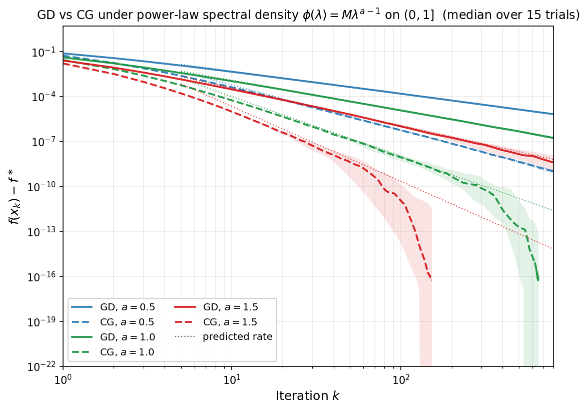
8. Stochastic Gradient Descent for Least Squares
All the algorithms studied so far—gradient descent, Chebyshev-accelerated gradient descent, and CG—access the matrix $A$ only through matrix-vector products $v\mapsto Av$. For the canonical least squares problem
\[\min_{x\in \mathbb{R}^d} f(x):=\tfrac{1}{2n}\|Dx-y\|^2,\]each such matrix vector product requires access to every row of $D\in \mathbb{R}^{n\times d}$ and requires $O(nd)$ basic arithmetic operations. When the dataset is large, this can be prohibitively expensive, and the runtime is dominated by data access rather than by the number of iterations.
The natural alternative is stochastic gradient descent (SGD), which at each step replaces the full gradient by a cheap unbiased estimator computed from a single data point, or a small batch. In this section, we analyze the performance of this algorithm.
Setup
Let $(x,y) \in \mathbb{R}^d \times \mathbb{R}$ be drawn from a distribution $\mathcal{D}$. The simplest example is when $\mathcal{D}$ is a uniform distribution over finitely many points. and consider the population square loss
\[L(w) = \tfrac{1}{2}\,\mathbb{E}\bigl[(y - \langle w, x\rangle)^2\bigr], \qquad w \in \mathbb{R}^d.\]We define the matrix
\[H := \mathbb{E}[xx^\top] \qquad\textrm{and set}\qquad \mu := \lambda_{\min}(H).\]We assume $H \succ 0$ throughout the section. As usual, for a vector $u$, we will use the norm $\lVert u\rVert _H^2 := u^\top H u$ induced by $H$. Exactly as in the deterministic least squares problem of Section 1 under the identification $A=H$, the excess population risk is the exact quadratic form
\[L(w) - L(w_\ast) = \tfrac{1}{2}\|w - w_\ast\|_H^2.\]We impose a single fourth-moment bound on the feature vectors: there is a constant $R > 0$ satisfying the condition
\[\mathbb{E}\bigl[\|x\|^2\, xx^\top\bigr] \;\preceq\; R^2\, H. \tag{25}\]This section in essence asserts that a type of fourth moment of $x$ is bounded by the second moment. Three standard settings where $(25)$ holds are the following:
- Bounded features. If $\lVert x\rVert \le R$ almost surely, then $(25)$ holds.
- Gaussian features. If $x \sim \mathcal{N}(0, H)$, then Isserlis’ formula gives \(\mathbb{E}[\|x\|^2\, xx^\top] = (\operatorname{Tr} H)\,H + 2H^2,\) and therefore $(25)$ holds with $R^2 = \operatorname{Tr} H + 2\lVert H\rVert _{\mathrm{op}} \le 3\operatorname{Tr}(H)$.
- Whitened features. Suppose $x = H^{1/2} z$, where the coordinates of $z$ are i.i.d., centered, have unit variance, and have kurtosis $\kappa = \mathbb{E} z_i^4 < \infty$. Then an elementary algebraic manipulations give
and therefore $(25)$ holds with $R^2 = \operatorname{Tr} H + (\kappa - 1)\lVert H\rVert _{\mathrm{op}}$.
Taking traces in $(25)$ yields $\operatorname{Tr}(H) = \mathbb{E}\lVert x\rVert ^2 \le R^2$, and in particular $H \preceq R^2 I$; thus $R^2$ upper bounds the top eigenvalue of $H$, and will play a role analogous to $\beta$ in Section 1.
Constant-stepsize SGD is the algorithm
\[w_t = w_{t-1} + \gamma\,(y_t - \langle w_{t-1}, x_t\rangle)\,x_t, \qquad t=1,2,\ldots, \tag{26}\]where $(x_t,y_t)$ are i.i.d. copies of $(x,y)$ and the stepsize satisfies $0 < \gamma < 1/R^2$. In contrast to the deterministic gradient method, the iterates $w_t$ do not converge to $w_\ast$; instead they contract exponentially to a noise floor proportional to $\gamma$ and oscillate around it. The size of this floor is governed by the covariance of the stochastic gradient at the minimizer. Define
\[\Sigma := \mathbb{E}\bigl[(y - \langle w_\ast, x\rangle)^2\, xx^\top\bigr], \quad \sigma_{\mathrm{MLE}}^2 := \tfrac{1}{2}\operatorname{Tr}(H^{-1}\Sigma), \quad \rho_{\mathrm{misspec}} := \frac{d\,\lVert H^{-1/2}\Sigma H^{-1/2}\rVert_{\mathrm{op}}}{\operatorname{Tr}(H^{-1}\Sigma)}.\]The misspecification parameter $\rho_{\mathrm{misspec}}$ takes values in $[1,d]$ and measures how far the problem is from well specified. In particular, it equals $1$ in the additive-noise model $y = \langle w_\ast, x\rangle + \eta$ with $\eta$ independent of $x$ and $\mathbb{E}[\eta^2]=\sigma^2$ (since then $\Sigma = \sigma^2 H$). The following theorem quantifies last-iterate behavior of the SGD.
Theorem 8.1 (Last-iterate constant-stepsize SGD). Under assumption $(25)$, strong convexity $H \succeq \mu I$ for some $\mu>0$, and with stepsize $0 < \gamma < 1/R^2$, the iterates $(26)$ satisfy
\[\mathbb{E}[L(w_t)] - L(w_\ast) \;\leq\; \underbrace{e^{-\gamma \mu t}\,R^2\,\lVert w_0-w_\ast\rVert^2}_{\text{bias}} \;+\; \underbrace{\frac{\gamma\,\operatorname{Tr}(\Sigma)}{2-\gamma R^2}}_{\text{noise floor}}. \tag{27}\]Proof. The first-order optimality condition $\nabla L(w_\ast)=0$ reads $\mathbb{E}[(y - \langle w_\ast, x\rangle)x]=0$. Set $e_t := w_t - w_\ast$, $B_t := I - \gamma x_t x_t^\top$, and $\xi_t := -(y_t - \langle w_\ast, x_t\rangle)x_t$. Then we have $\mathbb{E}[\xi_t]=0$, $\mathbb{E}[\xi_t\xi_t^\top]=\Sigma$, and elementary algebra shows that $(26)$ becomes the recursion
\[e_t = B_t\,e_{t-1} - \gamma\,\xi_t. \tag{28}\]Because this recursion is linear, we decompose $e_t = b_t + v_t$ into the bias process $b_t$, which propagates the initial error $w_0 - w_\ast$ through the noiseless part of the recursion, and the variance process $v_t$, which accumulates the gradient noise $\xi_1,\ldots,\xi_t$ starting from zero:
\[\begin{aligned} b_0 &= w_0 - w_\ast, &\qquad b_t &= B_t\,b_{t-1} &&\text{for all } t\geq 1,\\ v_0 &= 0, &\qquad v_t &= B_t\,v_{t-1} - \gamma\,\xi_t &&\text{for all } t\geq 1. \end{aligned} \tag{29}\]Adding the two recursions gives $b_t + v_t = B_t(b_{t-1} + v_{t-1}) - \gamma\,\xi_t$ with $b_0 + v_0 = w_0 - w_\ast = e_0$, so by induction $e_t = b_t + v_t$ as claimed. Note that $b_t$ depends only on the features $x_1,\ldots,x_t$ (through the contractions $B_s$) and the fixed initial error, while $v_t$ depends on the gradient-noise terms $\xi_1,\ldots,\xi_t$. Note that since $v_0=0$ and $\mathbb{E}[\xi_t]=0$, induction immediately gives $\mathbb{E}[v_t]=0$ for all $t$.
Since $L(w) - L(w_\ast) = \tfrac{1}{2}\lVert w-w_\ast\rVert_H^2$, the elementary inequality $\lVert a+b\rVert_H^2 \le 2\lVert a\rVert_H^2 + 2\lVert b\rVert_H^2$ applied to $e_t = b_t + v_t$ gives
\[\mathbb{E}[L(w_t)] - L(w_\ast) \;=\; \tfrac{1}{2}\mathbb{E}\lVert e_t\rVert_H^2 \;\leq\; \mathbb{E}\lVert b_t\rVert_H^2 \;+\; \mathbb{E}\lVert v_t\rVert_H^2,\]so it suffices to bound the two terms on the right.
Bias contraction. Conditioning on the past in the bias recursion and expanding the square yields
\[\begin{aligned} \mathbb{E}\bigl[\lVert b_t\rVert^2 \mid b_{t-1}\bigr] &\;=\;\mathbb{E}\bigl[\lVert (I-\gamma\,xx^{\top})\,b_{t-1}\rVert^2 \mid b_{t-1}\bigr] \\ &\;=\; \lVert b_{t-1}\rVert^2 \;-\; 2\gamma\,b_{t-1}^\top H\,b_{t-1} \;+\; \gamma^2\,b_{t-1}^\top\underbrace{\mathbb{E}[\lVert x\rVert^2\,xx^\top]}_{\preceq\,R^2 H}\,b_{t-1}. \end{aligned}\]Applying the fourth-moment bound $(25)$ in the last term replaces $\mathbb{E}[\lVert x\rVert^2 xx^\top]$ by $R^2 H$ and collapses the two $H$-quadratic forms, giving
\[\mathbb{E}\bigl[\lVert b_t\rVert^2\mid b_{t-1}\bigr] \;\leq\; \lVert b_{t-1}\rVert^2 \;-\; \gamma\bigl(2 - \gamma R^2\bigr)\,b_{t-1}^\top H\,b_{t-1}.\]Since $\gamma R^2 < 1$ gives $2 - \gamma R^2 \ge 1$, and strong convexity $H \succeq \mu I$ gives $b_{t-1}^\top H\,b_{t-1} \ge \mu\,\lVert b_{t-1}\rVert^2$, we obtain the one-step contraction
\[\mathbb{E}\bigl[\lVert b_t\rVert^2\mid b_{t-1}\bigr] \;\leq\; \lVert b_{t-1}\rVert^2 \;-\; \gamma\,b_{t-1}^\top H\,b_{t-1} \;\leq\; (1 - \gamma\mu)\,\lVert b_{t-1}\rVert^2.\]Taking total expectation, using the tower rule, and iterating from $b_0 = w_0 - w_\ast$, yields
\[\mathbb{E}\lVert b_t\rVert^2 \;\leq\; (1-\gamma\mu)^t\,\lVert w_0 - w_\ast\rVert^2 \;\leq\; e^{-\gamma\mu t}\,\lVert w_0 - w_\ast\rVert^2.\]Finally, combining with the operator bound $H \preceq R^2 I$ (a consequence of $\operatorname{Tr}(H) = \mathbb{E}\lVert x\rVert^2 \le R^2$) converts the $\ell^2$ bound into the $H$-weighted one,
\[\mathbb{E}\lVert b_t\rVert_H^2 \;=\; \mathbb{E}[b_t^\top H\,b_t] \;\leq\; R^2\,\mathbb{E}\lVert b_t\rVert^2 \;\leq\; R^2\,e^{-\gamma\mu t}\,\lVert w_0 - w_\ast\rVert^2. \tag{30}\]Variance floor. Set $C_t := \mathbb{E}[v_t v_t^\top]$. Squaring the variance recursion gives
\[v_t v_t^\top \;=\; B_t\,v_{t-1}v_{t-1}^\top\,B_t^\top \;-\; \gamma\,B_t v_{t-1}\xi_t^\top \;-\; \gamma\,\xi_t v_{t-1}^\top B_t^\top \;+\; \gamma^2\,\xi_t\xi_t^\top.\]We claim that the two cross terms have zero mean. The key facts are that $v_{t-1}$ depends only on $(x_1,\xi_1),\dots,(x_{t-1},\xi_{t-1})$ and is therefore independent of the fresh data $(x_t,y_t)$, and that $\mathbb{E}[\xi_t] = \nabla L(w_\ast) = 0$ by definition of $w_\ast$. Conditioning on $v_{t-1}$ and taking the expectation over $(x_t,y_t)$ gives
\[\begin{aligned} \mathbb{E}\bigl[B_t\,v_{t-1}\xi_t^\top \,\big|\, v_{t-1}\bigr] &= \mathbb{E}\bigl[(I-\gamma x_tx_t^\top)\,v_{t-1}\,\xi_t^\top \,\big|\, v_{t-1}\bigr] \\ &= v_{t-1}\,\mathbb{E}[\xi_t]^\top - \gamma\,\mathbb{E}\bigl[x_tx_t^\top v_{t-1}\,\xi_t^\top \,\big|\, v_{t-1}\bigr] \\ &= -\gamma\,\mathbb{E}\bigl[(v_{t-1}^\top x_t)\,x_t\,\xi_t^\top \,\big|\, v_{t-1}\bigr], \end{aligned}\]where the last line uses $\mathbb{E}[\xi_t]=0$ and $x_tx_t^\top v_{t-1}=(v_{t-1}^\top x_t)x_t$. The last line is linear in $v_{t-1}$. Thus taking the outer expectation over $v_{t-1}$ replaces $v_{t-1}$ by $\mathbb{E}[v_{t-1}]=0$. Therefore using the tower rule for expectations we deduce $\mathbb{E}[B_t\,v_{t-1}\xi_t^\top]=0$, as claimed.
Define the covariance $C_t:=\mathbb{E}[v_tv^{\top}_t]$ and the linear operator on matrices $\mathcal M(M) := \mathbb{E}[(I-\gamma xx^\top)\,M\,(I-\gamma xx^\top)]$. Then using the equality $\mathbb{E}[\xi_t\xi_t^\top] = \Sigma$, we obtain the key recursion for the covariance
\[C_t \;=\; \mathcal{M}(C_{t-1}) + \gamma^2\,\Sigma. \tag{31}\]We next show that the sequence $\lbrace C_t\rbrace$ is monotone in the PSD order. To see this, subtracting consecutive copies of $(31)$ gives $C_{t+1} - C_t = \mathcal{M}(C_t - C_{t-1})$. Therefore, by induction starting from $C_1 - C_0 = \gamma^2\Sigma \succeq 0$ and using that $\mathcal{M}$ preserves PSD order, every consecutive difference is PSD and therefore $C_t \preceq C_{t+1}$, as claimed.
Taking traces in $(31)$ and using the identity $\operatorname{Tr}((xx^\top)\,C\,(xx^\top)) = (x^\top Cx)\,\lVert x\rVert^2$ to simplify the resulting fourth-order term gives
\[\operatorname{Tr}(C_t) \;=\; \operatorname{Tr}(C_{t-1}) \;-\; 2\gamma\,\operatorname{Tr}(HC_{t-1}) \;+\; \gamma^2\,\mathbb{E}\bigl[(x^\top C_{t-1}x)\,\lVert x\rVert^2\bigr] \;+\; \gamma^2\,\operatorname{Tr}(\Sigma).\]The fourth-moment bound $(25)$ controls the third term via $\mathbb{E}[(x^\top Cx)\lVert x\rVert^2] = \operatorname{Tr}(C\,\mathbb{E}[\lVert x\rVert^2 xx^\top]) \le R^2\operatorname{Tr}(HC)$. Combined with $\gamma R^2 < 1$, so that $2-\gamma R^2 \ge 1$, and strong convexity $H \succeq \mu I$, so that $\operatorname{Tr}(HC_{t-1}) \ge \mu\operatorname{Tr}(C_{t-1})$, we obtain the one-step contraction
\[\operatorname{Tr}(C_t) \;\le\; (1-\gamma\mu)\,\operatorname{Tr}(C_{t-1}) \;+\; \gamma^2\,\operatorname{Tr}(\Sigma).\]Iterating from $C_0 = 0$ yields
\[\operatorname{Tr}(C_t) \;=\; \mathbb{E}\lVert v_t\rVert^2 \;\leq\; \frac{\gamma\,\operatorname{Tr}(\Sigma)}{\mu} \qquad\text{for all }t\ge 0.\]Taking into account that $C_t$ is nondecreasing in PSD order, we see that $C_t$ lies in the compact set of PSD matrices with trace bounded by $\gamma\operatorname{Tr}(\Sigma)/\mu$. Therefore the sequence admits a limit point $C_\infty \succeq 0$, and taking the trace and the limit in $(31)$ we deduce that $C_{\infty}$ satisfies
\[\operatorname{Tr}(C_\infty) \;=\; \operatorname{Tr}(\mathcal{M}(C_\infty)) + \gamma^2\operatorname{Tr}(\Sigma).\]Expanding $\mathcal{M}(C_\infty)$ and rearranging yields
\[2\operatorname{Tr}(HC_\infty) \;=\; \gamma\,\mathbb{E}\bigl[(x^\top C_\infty x)\lVert x\rVert^2\bigr] + \gamma\,\operatorname{Tr}(\Sigma).\]The fourth-moment assumption $(25)$ bounds
\[\mathbb{E}\bigl[(x^\top Cx)\lVert x\rVert^2\bigr] \;=\; \operatorname{Tr}\!\bigl(C\,\mathbb{E}[\lVert x\rVert^2 xx^\top]\bigr) \;\leq\; R^2\operatorname{Tr}(HC),\]so $2\operatorname{Tr}(HC_\infty) \le \gamma R^2\operatorname{Tr}(HC_\infty) + \gamma\operatorname{Tr}(\Sigma)$, and rearranging gives $\operatorname{Tr}(HC_\infty) \le \gamma\operatorname{Tr}(\Sigma)/(2-\gamma R^2)$. Since $C_t \preceq C_\infty$ in PSD order and $H \succeq 0$, we deduce
\[\mathbb{E}\lVert v_t\rVert_H^2 \;=\; \operatorname{Tr}(HC_t) \;\leq\; \operatorname{Tr}(HC_\infty) \;\leq\; \frac{\gamma\,\operatorname{Tr}(\Sigma)}{2 - \gamma R^2}.\]Combining the bias and variance bounds yields $(27)$. $\square$
The bound $(27)$ decomposes the excess risk into a bias term that contracts at the geometric rate $e^{-\gamma\mu t}$—exactly the rate GD with stepsize $\gamma$ would achieve on a $\mu$-strongly-convex quadratic—and a noise floor $\gamma\operatorname{Tr}(\Sigma)/(2-\gamma R^2)$ that is independent of $t$ and proportional to the stepsize. A smaller $\gamma$ lowers the floor but slows the contraction, while a larger $\gamma$ contracts faster to a correspondingly higher floor: a classical bias–variance trade-off that no single constant stepsize can avoid.
Numerical illustration. The figure below makes the two phases of $(27)$ visible on the well-specified isotropic Gaussian model $x \sim \mathcal{N}(0, I_d)$, $y = \langle w_\ast, x\rangle + \eta$ with $\eta \sim \mathcal{N}(0,\sigma^2)$, for which $H = I$, $\mu = 1$, $R^2 = d+2$, and $\operatorname{Tr}(\Sigma) = d\sigma^2$. Taking $d=20$, $\sigma=0.3$, $w_0=0$, and stepsizes $\gamma R^2 \in \lbrace 0.2,0.5,0.8\rbrace$, we plot the median over $80$ trials of the single-iterate excess risk $L(w_t)-L(w_\ast)$ together with its $10$–$90\%$ interquantile band, and the asymptotic noise floor $\gamma\operatorname{Tr}(\Sigma)/(2(2-\gamma R^2))$ (dotted), which is the stationary excess risk of SGD on this model and which the bound $(27)$ tracks up to a factor of two. Each run contracts exponentially at rate $e^{-\gamma\mu t}$ until it reaches the stepsize-dependent floor, around which it then oscillates; smaller $\gamma$ gives a lower floor but a slower approach.
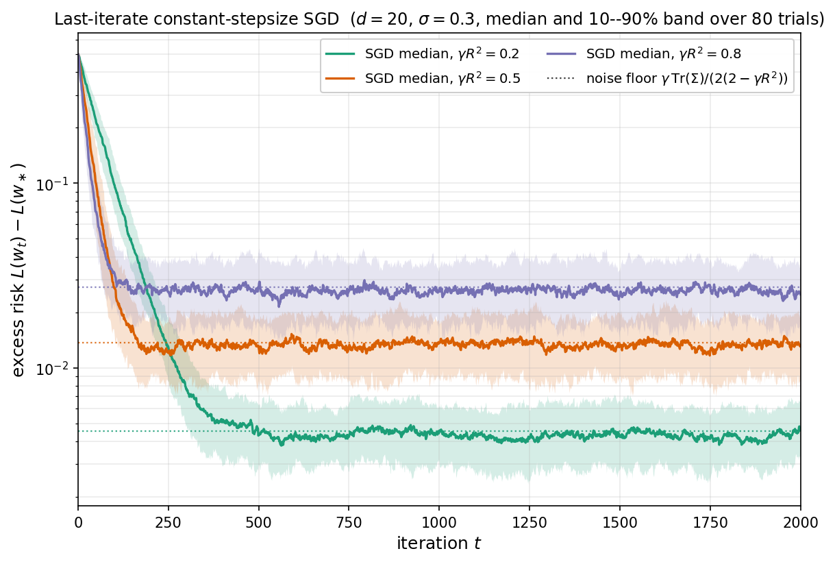
Even though the function values along the last iterate do not converge to the minimal values, we will see now that surprisingly, the function values do converge when measured along the average iterate. More precisely, define the tail average
\[\overline{w}_{t:T} \;:=\; \frac{1}{T - t}\sum_{s=t}^{T-1} w_s, \qquad 0 \le t < T.\]The cutoff $t$ discards a burn-in phase during which the iterates are still contracting toward $w_\ast$; averaging over $[t,T)$ then suppresses the variance below the floor of Theorem 8.1, as the next result shows.
Theorem 8.2 (Tail-averaged constant-stepsize SGD). Under assumption $(25)$ and with stepsize $0 < \gamma < 1/R^2$, the tail-averaged SGD iterates of $(26)$ satisfy
\[\mathbb{E}[L(\overline w_{t:T})] - L(w_\ast) \;\leq\; \underbrace{e^{-\gamma \mu t}\,R^2\,\|w_0-w_\ast\|^2}_{\text{bias}} \;+\; \underbrace{2\Big(1 + \tfrac{\gamma R^2}{1-\gamma R^2}\,\rho_{\mathrm{misspec}}\Big)\,\frac{\sigma_{\mathrm{MLE}}^2}{T-t}}_{\text{variance}}. \tag{32}\]The bound $(32)$ displays the classical bias–variance tradeoff of stochastic least squares. The bias contracts at the linear rate $e^{-\gamma \mu t}$—exactly the GD rate of Corollary 2.2 with $R^2$ in place of $\beta$—and decays with the burn-in length $t$. The variance, in contrast, is independent of the initialization and decays only as $1/(T-t)$ with the averaging window $T-t$, matching the statistically optimal rate. Choosing $t$ to be a constant fraction of $T$ (say $t = T/2$) therefore makes the bias negligible and recovers the $O(\sigma_{\mathrm{MLE}}^2/T)$ rate of the MLE.
Remark. In the well-specified additive-noise model $y = \langle w_\ast, x\rangle + \eta$, where $\eta$ is independent of $x$ with $\mathbb{E}[\eta]=0$ and $\mathbb{E}[\eta^2]=\sigma^2$, a direct computation gives $\Sigma = \sigma^2 H$, and hence $\sigma_{\mathrm{MLE}}^2 = \tfrac{1}{2}d\sigma^2$ and $\rho_{\mathrm{misspec}} = 1$. After a burn-in that makes the bias negligible, Theorem 8.2 reduces to $\mathbb{E}[L(\overline w_{t:T})] - L(w_\ast) \lesssim d\sigma^2/(T-t)$.
Numerical illustration. The figure below separates the two phases predicted by $(32)$ on the well-specified isotropic Gaussian model $x \sim \mathcal{N}(0, I_d)$, $y = \langle w_\ast, x\rangle + \eta$ with $\eta \sim \mathcal{N}(0,\sigma^2)$, taking $d=20$, $\sigma=0.3$, $w_0 = 0$, and stepsize $\gamma = \tfrac{1}{2}/(d+2)$ (so $\gamma R^2 = \tfrac12$). We plot the median over $60$ trials of the last-iterate risk $L(w_t) - L(w_\ast)$ and the tail-averaged risk $L(\overline w_{t/2:t}) - L(w_\ast)$ (shaded bands show the $10$–$90\%$ interquantile range), together with the bound $(32)$ specialized to burn-in $s=t/2$. The last iterate decays exponentially until it hits a noise floor on the order of $\gamma d\sigma^2$ and then stops improving, whereas the tail average keeps decaying at the $1/t$ rate. The theoretical bound $(32)$ upper-bounds the tail-averaged curve across the entire horizon.
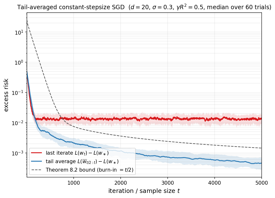
The animation below further visualizes the same comparison in two dimensions, on a fresh least-squares instance with $H = \mathrm{diag}(1, 0.25)$, $w_\ast = (2,-1)$, $w_0 = (-2.5, 2)$, $\sigma = 0.6$, stepsize $\gamma R^2 = 0.5$, and $T = 2000$ iterations (the viewport is zoomed onto $w_\ast$ and only every $100$th iterate is shown). All three methods run in the streaming setting of Theorems 8.1 and 8.2. Let us make the following observations, consistent with Theorems 8.1 and 8.2.
- GD glides smoothly down the contour ellipses and converges to $w_\ast$ at the geometric rate $e^{-\gamma\mu t}$.
- SGD’s last iterate contracts at the same geometric rate while it is far from $w_\ast$, but once it reaches a stepsize-dependent neighbourhood it is dominated by the gradient noise and oscillates around $w_\ast$ forever, never improving — this is precisely the noise floor in Theorem 8.1.
- The tail-averaged green curve smooths out the SGD oscillations and continues to drift toward $w_\ast$ as more iterates are absorbed into the average. By the end of the run it has tightened around $w_\ast$: its excess risk shrinks like $1/(T-t)$ rather than plateauing, exactly as Theorem 8.2 predicts.
Proof. We follow the setup of the proof of Theorem 8.1: the linear error recursion $(28)$, the bias–variance decomposition $(29)$, and the covariance recursion $(31)$. Write $\overline b_{t:T} := \tfrac{1}{T-t}\sum_{s=t}^{T-1} b_s$ and $\overline v_{t:T} := \tfrac{1}{T-t}\sum_{s=t}^{T-1} v_s$ for the tail averages of the bias and variance processes, so that $\overline w_{t:T} - w_\ast = \overline b_{t:T} + \overline v_{t:T}$. The elementary inequality $\lVert a+b\rVert_H^2 \le 2\lVert a\rVert_H^2 + 2\lVert b\rVert_H^2$ then yields
\[\mathbb{E}[L(\overline w_{t:T})] - L(w_\ast) \;=\; \tfrac{1}{2}\mathbb{E}\lVert\overline b_{t:T}+\overline v_{t:T}\rVert_H^2 \;\leq\; \mathbb{E}\lVert\overline b_{t:T}\rVert_H^2 \;+\; \mathbb{E}\lVert\overline v_{t:T}\rVert_H^2. \tag{33}\]We now bound each of the two summands.
Bias contraction. By Jensen’s inequality and the $H$-weighted bias bound $(30)$, we get
\[\mathbb{E}\lVert\overline b_{t:T}\rVert_H^2 \;\leq\; \frac{1}{T-t}\sum_{s=t}^{T-1}\mathbb{E}\lVert b_s\rVert_H^2 \;\leq\; R^2\,e^{-\gamma\mu t}\,\lVert w_0 - w_\ast\rVert^2. \tag{34}\]Variance averaging in terms of $C_\infty$. Set $A := I - \gamma H$, so that $0 \preceq A \preceq I$. Iterating the variance recursion in $(29)$ from $s$ to $r$ gives
\[v_r \;=\; \prod_{u=s+1}^{r}(I-\gamma x_u x_u^\top)\,v_s \;-\; \gamma\sum_{u=s+1}^{r}\Bigl(\prod_{j=u+1}^{r}(I-\gamma x_j x_j^\top)\Bigr)\,\xi_u,\]taking expectation conditional on $v_s$ eliminates the second term leaving the expression
\[\mathbb{E}[v_r\mid v_s]=A^{r-s}v_s.\]For $r \ge s$, the tower rule then yields the cross-covariance
\[\mathbb{E}[v_r v_s^\top] \;=\; \mathbb{E}\bigl[\mathbb{E}[v_r\mid v_s]\,v_s^\top\bigr] \;=\; \mathbb{E}\bigl[A^{r-s}v_s v_s^\top\bigr] \;=\; A^{r-s}\,C_s,\]where the second equality pulls the $v_s$-measurable factor $v_s^\top$ out of the conditional expectation and the third uses that $A^{r-s}$ is deterministic. For $r < s$, taking the transpose and using that $A = I - \gamma H$ and $C_r$ are symmetric gives $\mathbb{E}[v_r v_s^\top] = (\mathbb{E}[v_s v_r^\top])^\top = (A^{s-r}C_r)^\top = C_r A^{s-r}$. Now split the double sum $\mathbb{E}[\overline v_{t:T}\overline v_{t:T}^\top] = (T-t)^{-2}\sum_{r,s=t}^{T-1}\mathbb{E}[v_r v_s^\top]$ along $r > s$, $r = s$, $r < s$ and reindex each off-diagonal triangle by $\tau := \lvert r-s\rvert$. This produces the diagonal $\sum_s C_s$ and the symmetric off-diagonal contribution $\sum_s\sum_{\tau\ge 1}(A^\tau C_s + C_s A^\tau)$. At $\tau = 0$ the symmetric term $A^\tau C_s + C_s A^\tau$ equals $2C_s$, so extending the inner sum to $\tau \ge 0$ over-counts the diagonal by the PSD quantity $\sum_s C_s$; dropping this over-count yields the PSD upper bound
\[\mathbb{E}[\overline v_{t:T}\overline v_{t:T}^\top] \;\preceq\; \frac{1}{(T-t)^2}\sum_{s=t}^{T-1}\sum_{\tau=0}^{T-1-s}\bigl(A^\tau C_s + C_s A^\tau\bigr).\]Taking the $H$-trace and using that $A$ commutes with $H$, every $\operatorname{Tr}(HA^\tau C_s)$ is nonnegative, so we can extend the inner sum to all $\tau \geq 0$. The geometric series sums to $(I-A)^{-1} = (\gamma H)^{-1}$, and using $C_s \preceq C_\infty$ in PSD order we conclude
\[\mathbb{E}\lVert\overline v_{t:T}\rVert_H^2 \;\leq\; \frac{2\,\operatorname{Tr}(C_\infty)}{\gamma\,(T-t)}. \tag{35}\]Bounding the stationary covariance. Recall that the sequence $\lbrace C_t\rbrace$ is monotone in PSD order. Combined with the trace bound $\operatorname{Tr}(C_t) \le \gamma\operatorname{Tr}(\Sigma)/\mu$ from Theorem 8.1, this yields full convergence in $\mathbb{R}^{d\times d}$ to some $C_{\infty}$. To see this, for any $u \in \mathbb{R}^d$, the scalar $u^\top C_t u$ is nondecreasing and bounded, hence convergent. The polarization identity then extends this to convergence of every bilinear form $u^\top C_t v$, and taking $u, v$ to be standard basis vectors shows that $C_t$ converges entrywise to a limit $C_\infty \succeq 0$. Continuity of the linear map $\mathcal{M}$ then lets us pass to the limit in $(31)$ to obtain the matrix fixed-point
\[C_\infty = \mathcal{M}(C_\infty) + \gamma^2\Sigma,\]Expanding $\mathcal{M}$ and cancelling $C_\infty$ yields the matrix equation
\[HC_\infty + C_\infty H \;=\; \gamma\,\mathcal{S}(C_\infty) + \gamma\,\Sigma, \qquad \text{where}\quad \mathcal{S}(M) := \mathbb{E}\bigl[(x^\top M x)\,xx^\top\bigr]. \tag{36}\]Introduce now the auxiliary operator
\[\widetilde{\mathcal{T}}(M) := HM + MH - \gamma HMH.\]In particular, we may rewrite $(36)$ as
\[\widetilde{\mathcal{T}}(C_\infty) = \gamma\mathcal{S}(C_\infty) + \gamma\Sigma - \gamma HC_\infty H\]and dropping the last PSD term yields
\[\widetilde{\mathcal{T}}(C_\infty) \preceq \gamma\mathcal{S}(C_\infty) + \gamma\Sigma.\]By the helper Lemma 8.3 below (applied with $A = I - \gamma H$), the operator $\widetilde{\mathcal{T}}$ admits the explicit, PSD-monotone inverse
\[\widetilde{\mathcal{T}}^{-1}(M) \;=\; \gamma\sum_{k\ge 0} A^k\, M\, A^k. \tag{37}\]Applying $\widetilde{\mathcal{T}}^{-1}$ to both sides preserves the PSD ordering by Lemma 8.3, and yields
\[C_\infty \;\preceq\; \underbrace{\gamma\,\widetilde{\mathcal{T}}^{-1}\mathcal{S}(C_\infty)}_{=:\,\mathcal{P}(C_\infty)} + \gamma\,\widetilde{\mathcal{T}}^{-1}(\Sigma). \tag{38}\]Define now $\lVert \Sigma\rVert _H := \lVert H^{-1/2}\Sigma H^{-1/2}\rVert _{\mathrm{op}}$ and note that we trivially have $\Sigma \preceq \lVert \Sigma\rVert _H\,H$. From the formula $(37)$ for $\widetilde{\mathcal{T}}^{-1}$ and the fact that $A$ commutes with $H$, we obtain
\[\widetilde{\mathcal{T}}^{-1}H \;=\; \gamma\sum_{k\ge 0}A^{2k}H \;\preceq\; \gamma\sum_{k\ge 0}A^{k}H \;=\; I,\]and applying the PSD-preserving inverse $\widetilde{\mathcal{T}}^{-1}$ from Lemma 8.3 to the inequality $\Sigma \preceq \lVert\Sigma\rVert_H\,H$ gives $\widetilde{\mathcal{T}}^{-1}\Sigma \preceq \lVert \Sigma\rVert _H\,\widetilde{\mathcal{T}}^{-1}H \preceq \lVert \Sigma\rVert _H\,I$. The operator $\mathcal{S}$ is linear and PSD-monotone, so combined with the fourth-moment bound $(25)$, every $M$ with $0 \preceq M \preceq aI$ satisfies $\mathcal{S}(M) \preceq a\,\mathcal{S}(I) \preceq aR^2 H$. Applying the PSD-preserving inverse $\widetilde{\mathcal{T}}^{-1}$ and using the bound $\widetilde{\mathcal{T}}^{-1}H \preceq I$ gives
\[\mathcal{P}(M) \;=\; \gamma\,\widetilde{\mathcal{T}}^{-1}\mathcal{S}(M) \;\preceq\; a\gamma R^2\,\widetilde{\mathcal{T}}^{-1}H \;\preceq\; a\gamma R^2\,I. \tag{39}\]Iterating $(38)$ unfolds $C_\infty$ as
\[C_\infty \;\preceq\; \mathcal{P}^{k+1}(C_\infty) \;+\; \gamma\sum_{j=0}^{k}\mathcal{P}^{j}\bigl(\widetilde{\mathcal{T}}^{-1}\Sigma\bigr) \qquad \text{for every } k\ge 0,\]obtained by applying the PSD-monotone operator $\mathcal{P}$ to $(38)$ and substituting back. The contraction $(39)$ propagates through powers of $\mathcal{P}$. We apply this in two ways. First, since $C_\infty \preceq \operatorname{Tr}(C_\infty)\,I$, we get
\[\mathcal{P}^{k+1}(C_\infty) \;\preceq\; \operatorname{Tr}(C_\infty)\,(\gamma R^2)^{k+1}\,I \;\xrightarrow[k\to\infty]{}\; 0,\]so the residual term vanishes. Second, since $\widetilde{\mathcal{T}}^{-1}\Sigma \preceq \lVert\Sigma\rVert_H\,I$ from above, the geometric series satisfies
\[\gamma\sum_{j=0}^{\infty}\mathcal{P}^{j}\bigl(\widetilde{\mathcal{T}}^{-1}\Sigma\bigr) \;\preceq\; \gamma\,\lVert\Sigma\rVert_H\sum_{j=0}^{\infty}(\gamma R^2)^{j}\,I \;=\; \frac{\gamma\,\lVert\Sigma\rVert_H}{1-\gamma R^2}\,I.\]Letting $k\to\infty$ therefore yields the crude operator bound
\[C_\infty \;\preceq\; \frac{\gamma\,\lVert\Sigma\rVert_H}{1 - \gamma R^2}\,I. \tag{40}\]To sharpen $(40)$ to a trace bound we plug back into the matrix Lyapunov equation $(36)$. The operator bound $(40)$ together with PSD-monotonicity and linearity of $\mathcal{S}$ gives
\[\mathcal{S}(C_\infty) \;\preceq\; \frac{\gamma\,\lVert\Sigma\rVert_H}{1-\gamma R^2}\,\mathcal{S}(I) \;\preceq\; \frac{\gamma R^2\,\lVert\Sigma\rVert_H}{1-\gamma R^2}\,H,\]where the second inequality is $\mathcal{S}(I) \preceq R^2 H$ from $(25)$. Multiplying $(36)$ on the left by $H^{-1}$ and taking traces, the left-hand side becomes
\[\operatorname{Tr}\bigl(H^{-1}(HC_\infty + C_\infty H)\bigr) \;=\; \operatorname{Tr}(C_\infty) + \operatorname{Tr}(H^{-1}C_\infty H) \;=\; 2\operatorname{Tr}(C_\infty),\]For the right-hand side, $\gamma\operatorname{Tr}(H^{-1}\Sigma)$ stays as is, and the bound on $\mathcal{S}(C_\infty)$ is
\[\gamma\operatorname{Tr}\bigl(H^{-1}\mathcal{S}(C_\infty)\bigr) \;\leq\; \frac{\gamma^2 R^2\,\lVert\Sigma\rVert_H}{1-\gamma R^2}\,\operatorname{Tr}(H^{-1}H) \;=\; \frac{\gamma^2 R^2\,d\,\lVert\Sigma\rVert_H}{1-\gamma R^2}.\]We thus arrive at the estimate
\[2\operatorname{Tr}(C_\infty) \;\leq\; \gamma\operatorname{Tr}(H^{-1}\Sigma) + \frac{\gamma^2 R^2\,d\,\lVert\Sigma\rVert_H}{1-\gamma R^2}.\]Substituting into $(35)$ and recognizing $\sigma_{\mathrm{MLE}}^2 = \tfrac12\operatorname{Tr}(H^{-1}\Sigma)$ and $\rho_{\mathrm{misspec}} = d\,\lVert\Sigma\rVert_H/\operatorname{Tr}(H^{-1}\Sigma)$ yields the final variance bound
\[\mathbb{E}\lVert\overline v_{t:T}\rVert_H^2 \;\leq\; 2\Big(1 + \frac{\gamma R^2}{1-\gamma R^2}\,\rho_{\mathrm{misspec}}\Big)\frac{\sigma_{\mathrm{MLE}}^2}{T-t}. \tag{41}\]Combining the bias bound $(34)$ and the variance bound $(41)$ with the decomposition $(33)$ produces $(32)$. $\square$
It remains to record the algebraic fact about $\widetilde{\mathcal{T}}$ used in the proof above.
Lemma 8.3 (Inverse of $\widetilde{\mathcal{T}}$). Let $H$ be a symmetric positive definite matrix and $\gamma > 0$ with $\gamma\lVert H\rVert_{\mathrm{op}} < 1$. Set $A := I - \gamma H$ and define the linear operator on symmetric matrices
\[\widetilde{\mathcal{T}}(M) := HM + MH - \gamma HMH.\]Then $\widetilde{\mathcal{T}}$ is invertible with
\[\widetilde{\mathcal{T}}^{-1}(M) \;=\; \gamma\sum_{k=0}^{\infty} A^k\, M\, A^k.\]Proof. Expand $A M A = (I-\gamma H)\,M\,(I-\gamma H) = M - \gamma HM - \gamma MH + \gamma^2 HMH$, so that
\[M - AMA \;=\; \gamma\bigl(HM + MH - \gamma HMH\bigr) \;=\; \gamma\,\widetilde{\mathcal{T}}(M). \tag{42}\]The hypothesis $\gamma\lVert H\rVert_{\mathrm{op}}<1$ together with $H \succ 0$ yields $0 \prec A \prec I$ and therefore the series
\[\Phi(M) \;:=\; \gamma\sum_{k\ge 0}A^k\,M\,A^k\]converges absolutely. Applying $(42)$ with $M$ replaced by $\Phi(M)$ and reindexing gives the telescoping identity
\[\widetilde{\mathcal{T}}\bigl(\Phi(M)\bigr) \;=\; \tfrac{1}{\gamma}\bigl(\Phi(M) - A\,\Phi(M)\,A\bigr) \;=\; \sum_{k\ge 0}A^k M A^k - \sum_{k\ge 1}A^k M A^k \;=\; M.\]The same calculation with the order of $\Phi$ and $\widetilde{\mathcal{T}}$ reversed gives $\Phi\bigl(\widetilde{\mathcal{T}}(M)\bigr) = M$, so $\Phi = \widetilde{\mathcal{T}}^{-1}$, completing the proof. $\square$
The variance term $\sigma_{\mathrm{MLE}}^2/(T-t)$ in Theorem 8.2 is in fact sharp: no algorithm processing $T$ stochastic samples can do better than the $\sigma^2 d/T$ rate that tail-averaged constant-stepsize SGD already achieves. The matching lower bound, due to Mourtada [Mou22], is proved in §9.
Mini-batches, saturation, and the critical batch size
In practice each step of $(26)$ is replaced by an average over a small mini-batch of $B$ samples. This raises an immediate question: how does the bound of Theorem 8.2 change with $B$, and how large should $B$ be? The answer is essentially read off the variance term, and uncovers the phenomenon of batch saturation: once the noise has been driven below the remaining optimization bias, additional samples per step buy nothing. To keep the formulas readable we fix the stepsize at $\gamma R^2 = \tfrac{1}{2}$ throughout this section, so that $\gamma R^2/(1-\gamma R^2) = 1$ and the variance prefactor of $(32)$ collapses to $2(1+\rho_{\mathrm{misspec}})$.
For an integer $B \geq 1$, the mini-batch variant of $(26)$ takes the step
\[w_t \;=\; w_{t-1} + \frac{\gamma}{B}\sum_{j=1}^{B}\bigl(y_{t,j}-\langle w_{t-1},x_{t,j}\rangle\bigr)\,x_{t,j},\]with $(x_{t,j},y_{t,j})$ independent copies of $(x,y)$. Setting
\[\widehat H_t \;:=\; \frac{1}{B}\sum_{j=1}^{B} x_{t,j}x_{t,j}^{\top}, \qquad \overline\xi_t \;:=\; -\frac{1}{B}\sum_{j=1}^{B}\bigl(y_{t,j}-\langle w_\ast,x_{t,j}\rangle\bigr)\,x_{t,j},\]the error $w_t - w_\ast$ obeys the same linear recursion as in $(28)$, with $xx^\top$ replaced by the empirical average $\widehat H_t$ and the noise covariance scaled by $1/B$:
\[w_t - w_\ast \;=\; (I-\gamma\widehat H_t)\,(w_{t-1}-w_\ast) \;-\; \gamma\,\overline\xi_t, \qquad \mathbb{E}[\widehat H_t] = H, \qquad \mathbb{E}[\overline\xi_t\overline\xi_t^\top] = \tfrac{1}{B}\,\Sigma.\]A short calculation, expanding $\widehat H_t^2$ and using independence, shows that the fourth-moment bound $\mathbb{E}[\widehat H_t^2] \preceq R^2 H$ continues to hold with the same constant $R^2$ as in $(25)$. Tracking the $1/B$ factor through the bias–variance proof of Theorem 8.2, and writing $\overline w_{t:T}^{(B)}$ for the resulting tail average, then gives the mini-batch tail-averaged bound
\[\mathbb{E}[L(\overline w_{t:T}^{(B)})] - L(w_\ast) \;\leq\; \underbrace{R^2\,e^{-\gamma\mu t}\,\|w_0-w_\ast\|^2}_{\text{bias}} \;+\; \underbrace{2(1+\rho_{\mathrm{misspec}})\,\frac{\sigma_{\mathrm{MLE}}^2}{B(T-t)}}_{\text{variance}}.\]The bias depends only on the number of parameter updates $t$, while the variance scales as $1/(B(T-t))$ in the total number of averaged samples. The two natural ways of using this bound correspond to the two natural resources in stochastic optimization: parallel time and sample budget.
Fixed-update regime. Suppose first that the parallel wall-clock budget $T$ is held fixed, so that a batch of $B$ samples is processed at the same cost as a single sample. The bias is then independent of $B$, while the variance decreases as $1/B$ until it falls below the bias. Equating the two terms at burn-in $t=T/2$ identifies the critical batch size
\[B_{\mathrm{crit}}(T) \;\approx\; \frac{(1+\rho_{\mathrm{misspec}})\,\sigma_{\mathrm{MLE}}^2}{T\,e^{-\gamma\mu T/2}\,R^2\,\|w_0-w_\ast\|^2}.\]For $B \ll B_{\mathrm{crit}}(T)$, doubling the batch roughly halves the excess risk; for $B \gg B_{\mathrm{crit}}(T)$ the variance is already negligible and the curve flattens at the deterministic bias level. This is batch saturation.
Fixed-sample regime. Suppose now that the total number of samples $N=BT$ is held fixed and the tail window is $t=T/2$, so that $B(T-t) = N/2$. The variance term then collapses to an $O(\sigma_{\mathrm{MLE}}^2/N)$ statistical floor that does not depend on $B$ at all, and only the bias depends on $B$, through $T = N/B$:
\[\mathbb{E}[L(\overline w_{T/2:T}^{(B)})] - L(w_\ast) \;\leq\; R^2\,\exp\!\Big(-\tfrac{\gamma\mu N}{2B}\Big)\,\|w_0-w_\ast\|^2 \;+\; \frac{4(1+\rho_{\mathrm{misspec}})\,\sigma_{\mathrm{MLE}}^2}{N}.\]The largest useful batch is the largest $B$ for which the bias is still on the order of the statistical floor, namely
\[B \;\lesssim\; \frac{\gamma\mu\,N}{\log\!\Big(\tfrac{R^2\,\|w_0-w_\ast\|^2\,N}{(1+\rho_{\mathrm{misspec}})\,\sigma_{\mathrm{MLE}}^2}\Big)}.\]Below this threshold the algorithm is statistically limited and any further reduction in error requires more samples; above it the algorithm is optimization limited, because too few updates have been spent removing the bias.
Numerical illustration. The figure below illustrates both regimes on the same well-specified isotropic Gaussian model used in Theorems 8.1 and 8.2, with $d=20$ and $\sigma=0.3$. For each batch size $B \in \lbrace 1,2,4,\ldots,512\rbrace$ we run constant-stepsize mini-batch SGD with burn-in $t=T/2$ and report the median, with a $10$–$90\%$ interquantile band, of the tail-averaged excess risk $L(\overline w_{T/2:T}^{(B)})-L(w_\ast)$ over $45$ trials. The left panel fixes the number of updates at $T=250$ and shows the fixed-update regime: the variance decays like $1/B$ until the curve flattens at the deterministic bias level around the predicted $B_{\mathrm{crit}}\approx 41$. The right panel fixes the total sample budget at $N=8192$ and shows the fixed-sample regime: the risk is essentially flat for moderate $B$, since the variance depends only on $N$, but rises sharply once $B$ is so large that $T=N/B$ is too small to absorb the bias.
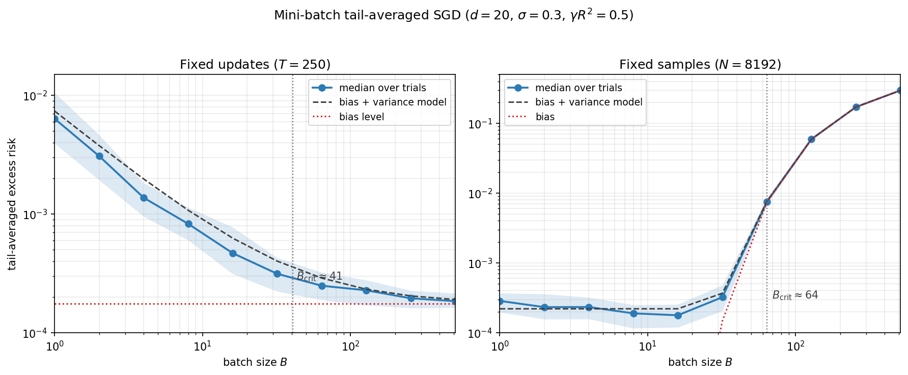
Theorem 8.1 is the classical last-iterate bound for constant-stepsize SGD on least squares and dates back to [RM51,Pol87,KY03]; the streamlined proof via the bias–variance decomposition and a Lyapunov equation for the stationary noise covariance is standard and appears, with variants, in e.g. [BM11, BM13, DB15, JKK+18]. Theorem 8.2 is due to Jain, Kakade, Kidambi, Netrapalli, Pillutla, and Sidford [JKK+18], who established minimax optimality of tail-averaged constant-stepsize SGD for least squares via a Markov-chain/covariance analysis. The matching minimax lower bound that confirms this optimality is the subject of §9.
Interpolation and the randomized Kaczmarz algorithm
Theorems 8.1 and 8.2 expressed the excess risk as a bias plus a noise floor, with the noise floor governed by the residual $y - \langle w_\ast, x\rangle$ at the minimizer. Interpolation is the limiting regime in which this residual vanishes:
\[y \;=\; \langle w_\ast, x\rangle \qquad \text{almost surely,}\]equivalently $\Sigma = \mathbb{E}[(y - \langle w_\ast, x\rangle)^2 xx^\top] = 0$ and $\sigma_{\mathrm{MLE}}^2 = 0$, so the noise floors in $(27)$ and $(32)$ disappear. Theorem 8.1 then specializes to a clean linear-rate statement.
Corollary 8.4 (SGD on interpolation problems). Suppose $y = \langle w_\ast, x\rangle$ almost surely, $H \succeq \mu I$ for some $\mu > 0$, and assumption $(25)$ holds. Then for any $0 < \gamma < 1/R^2$, the constant-stepsize iterates $(26)$ satisfy
\[\mathbb{E}[L(w_t)] - L(w_\ast) \;\leq\; e^{-\gamma\mu t}\,R^2\,\lVert w_0 - w_\ast\rVert^2.\]This is a sharp departure from the noisy regime: in interpolation, constant-stepsize SGD — with no averaging, no decreasing stepsize, and no batch growth — already achieves linear convergence, contracting at the per-step rate $\gamma\mu$, optimized to $\mu/R^2$ at $\gamma = 1/R^2$.
A canonical example is the discrete consistent linear system: given $D \in \mathbb{R}^{n\times d}$ with rows $d_1,\ldots,d_n$ and $y \in \mathbb{R}^n$ satisfying $y = D w_\ast$ for some $w_\ast$, Corollary 8.4 governs the constant-stepsize SGD iteration in which $(x,y) = (d_i, y_i)$ is sampled uniformly from $\lbrace 1,\ldots,n\rbrace$. In this setup $H = D^\top D / n$, $\mu = \sigma_{\min}^2(D)/n$, and the smallest valid $R^2$ in $(25)$ is $\max_i \lVert d_i\rVert^2$, so the optimal stepsize $\gamma = 1/R^2$ yields the SGD rate $\sigma_{\min}^2(D)/(n\,\max_i\lVert d_i\rVert^2)$.
A natural question is whether one can do better by exploiting the row geometry. The classical randomized Kaczmarz algorithm of Strohmer and Vershynin [SV09] does exactly this: it samples rows with norm-weighted probability and uses a row-adaptive stepsize that performs an exact orthogonal projection at each step.
Algorithm 2 (Randomized Kaczmarz)
Input: $D \in \mathbb{R}^{n\times d}$ with nonzero rows $d_1, \ldots, d_n$, $\;y \in \mathbb{R}^n$, $\;w_0 \in \mathbb{R}^d$
Set $p_i = \lVert d_i\rVert^2 / \lVert D\rVert_F^2$ for $i = 1, \ldots, n$
For $t = 0, 1, 2, \ldots$ do:
$\qquad$ sample $i_t \in \lbrace 1, \ldots, n\rbrace$ with probability $p_{i_t}$
$\qquad w_{t+1} = w_t \;+\; \dfrac{y_{i_t} - \langle d_{i_t}, w_t\rangle}{\lVert d_{i_t}\rVert^2}\,d_{i_t}$
Each update can be geometrically understood as an orthogonal projection: $w_{t+1}$ is the closest point to $w_t$ in the affine hyperplane $\lbrace w \in \mathbb{R}^d : \langle d_{i_t}, w\rangle = y_{i_t}\rbrace$. To make the geometry concrete, consider the 2D consistent system with $n=5$ unit-norm rows $d_1,\ldots,d_5 \in \mathbb{R}^2$ and right-hand side $y_i = \langle d_i, w_\ast\rangle$, so that the lines $\ell_i = \lbrace w \in \mathbb{R}^2 : \langle d_i, w\rangle = y_i\rbrace$ all pass through the common point $w_\ast$. Starting from a fixed $w_0$, each Kaczmarz step picks one of the five lines (uniformly, since $\lVert d_i\rVert = 1$) and replaces $w_t$ by its orthogonal projection onto that line. The animation below shows the first $14$ iterations: at each step the chosen line $\ell_{i_t}$ is drawn in red and the dashed arrow traces the projection from $w_t$ to $w_{t+1}$.
The following theorem captures the classical convergence guarantee.
Theorem 8.5 (Strohmer-Vershynin). Assume $D \in \mathbb{R}^{n\times d}$ has linearly independent columns and that $y = D w_\ast$. The randomized Kaczmarz iterates of Algorithm 2 satisfy
\[\mathbb{E}\,\lVert w_t - w_\ast\rVert^2 \;\leq\; \Big(1 - \frac{\sigma_{\min}^2(D)}{\lVert D\rVert_F^2}\Big)^t\,\lVert w_0 - w_\ast\rVert^2.\]Proof. Subtract $w_\ast$ from both sides of the Kaczmarz update and use the equality $y_{i_t} = \langle d_{i_t}, w_\ast\rangle$ to rewrite the residual as $y_{i_t} - \langle d_{i_t}, w_t\rangle = -\langle d_{i_t},\,w_t - w_\ast\rangle$, giving
\[w_{t+1} - w_\ast \;=\; (w_t - w_\ast) \;-\; \frac{\langle d_{i_t},\,w_t - w_\ast\rangle}{\lVert d_{i_t}\rVert^2}\,d_{i_t}.\]Squaring and expanding yields the estimate
\[\lVert w_{t+1} - w_\ast\rVert^2 \;=\; \lVert w_t - w_\ast\rVert^2 \;-\; 2\,\frac{\langle d_{i_t},\,w_t - w_\ast\rangle^2}{\lVert d_{i_t}\rVert^2} \;+\; \frac{\langle d_{i_t},\,w_t - w_\ast\rangle^2}{\lVert d_{i_t}\rVert^4}\,\lVert d_{i_t}\rVert^2,\]Combining the cross term and the last term, we therefore arrive at the expression
\[\lVert w_{t+1} - w_\ast\rVert^2 \;=\; \lVert w_t - w_\ast\rVert^2 \;-\; \frac{\langle d_{i_t},\, w_t - w_\ast\rangle^2}{\lVert d_{i_t}\rVert^2}.\]Taking conditional expectation over $i_t \sim p$, we obtain
\[\mathbb{E}\bigl[\lVert w_{t+1}-w_\ast\rVert^2 \,\big|\, w_t\bigr] \;=\; \lVert w_t - w_\ast\rVert^2 \;-\; \frac{1}{\lVert D\rVert_F^2}\sum_{i=1}^n \langle d_i,\,w_t - w_\ast\rangle^2 \;=\; \lVert w_t - w_\ast\rVert^2 \;-\; \frac{\lVert D(w_t - w_\ast)\rVert^2}{\lVert D\rVert_F^2}.\]Linear independence of the columns of $D$ yields $\lVert Du\rVert^2 \geq \sigma_{\min}^2(D)\,\lVert u\rVert^2$ for every $u \in \mathbb{R}^d$, so
\[\mathbb{E}\bigl[\lVert w_{t+1}-w_\ast\rVert^2 \,\big|\, w_t\bigr] \;\leq\; \Big(1 - \frac{\sigma_{\min}^2(D)}{\lVert D\rVert_F^2}\Big)\,\lVert w_t - w_\ast\rVert^2.\]Iterating this one-step contraction from $t=0$ produces the claim. $\square$
Comparison with SGD. Writing $\overline{\lVert d\rVert^2} := \tfrac{1}{n}\sum_i\lVert d_i\rVert^2$ for the average squared row norm, the Kaczmarz rate of Theorem 8.5 reads $\sigma_{\min}^2(D)/\lVert D\rVert_F^2 = \sigma_{\min}^2(D)/(n\,\overline{\lVert d\rVert^2})$. Lining this up with the SGD rate derived above, we obtain the comparison
\[\underbrace{\frac{\sigma_{\min}^2(D)}{n\,\max_i\lVert d_i\rVert^2}}_{\text{SGD (uniform sampling)}} \;\leq\; \underbrace{\frac{\sigma_{\min}^2(D)}{n\,\overline{\lVert d\rVert^2}}}_{\text{Kaczmarz}},\]Note that we are only comparing upper-bounds on performance. Nonetheless, the comparison is meaningful. The difference between the two bound is whether the worst or the average squared row norm appears in the denominator. The two coincide when all row norms are equal; the Kaczmarz rate dominates by the row-norm spread $\max_i\lVert d_i\rVert^2 / \overline{\lVert d\rVert^2}$, which can be arbitrarily large when the rows are scaled very differently. Behind the gain is a small algorithmic shift: Kaczmarz draws rows with norm-weighted probability rather than uniformly, and uses the row-adaptive stepsize $1/\lVert d_{i_t}\rVert^2$ rather than the global $1/\max_i\lVert d_i\rVert^2$. Together these two adjustments swap $\max_i\lVert d_i\rVert^2$ for $\overline{\lVert d\rVert^2}$ in the per-step contraction.
Remark (why not just solve a smaller linear subsystem?). A natural alternative to Kaczmarz is to pick a small subset of $m \geq d$ rows of $D$ and solve the reduced system $D_S w = y_S$ directly. Deterministic row selection is delicate: an arbitrary $d$-row submatrix can have a much smaller minimum singular value than $D$ itself, and finding a well-conditioned subset is hard in general (the column-subset-selection problem). The randomized version — random row sampling — leads to a different class of techniques called sketching. The two techniques are largely complementary.
Remark (why not rescale rows and run standard SGD?). Another tempting reduction is to renormalize each equation, $\tilde d_i := d_i/\lVert d_i\rVert$ and $\tilde y_i := y_i/\lVert d_i\rVert$, so that the rescaled system $\tilde D w = \tilde y$ has unit-norm rows. The rescaling also changes the stepsize prescribed by Theorem 8.1: the smallest valid $R^2$ is now $\tilde R^2 = \max_i\lVert\tilde d_i\rVert^2 = 1$, so the optimal stepsize on the rescaled problem is $\gamma = 1/\tilde R^2 = 1$ rather than the smaller $1/\max_i\lVert d_i\rVert^2$ used on the original. With this prescribed stepsize, standard SGD on $\tilde D w = \tilde y$ produces the update
\[w_{t+1} = w_t + (\tilde y_{i_t} - \langle \tilde d_{i_t}, w_t\rangle)\,\tilde d_{i_t} \;=\; w_t + \frac{y_{i_t} - \langle d_{i_t}, w_t\rangle}{\lVert d_{i_t}\rVert^2}\,d_{i_t},\]which is the Kaczmarz projection step. Indeed, this is exactly Algorithm 2 applied to the rescaled system $(\tilde D,\tilde y)$, since the norm-weighted distribution $p_i = \lVert\tilde d_i\rVert^2/\lVert\tilde D\rVert_F^2$ collapses to uniform when all rows have unit norm. So the question is which system one applies the projection update to: the original $(D,y)$, where the norm-weighted distribution favors long rows, or the rescaled $(\tilde D,\tilde y)$, where every row is sampled equally. The two are different algorithms, and Theorem 8.5 gives correspondingly different rates: $\sigma_{\min}^2(D)/\lVert D\rVert_F^2$ on the original, $\sigma_{\min}^2(\tilde D)/n$ on the rescaled. The rescaling can either improve or degrade $\sigma_{\min}$, so neither variant dominates the other in general.
Numerical illustration. The figure below compares the three algorithms above — uniform-sampling SGD on $D$ with stepsize $\gamma = 1/\max_i\lVert d_i\rVert^2$, uniform-sampling SGD on the row-rescaled system $\tilde D, \tilde y$ with stepsize $\gamma = 1$, and randomized Kaczmarz — on a synthetic interpolation least-squares instance with $n=500$, $d=50$, and rows $d_i \sim \mathcal{N}(0, I_d)$ rescaled so that the row norms span a multiplicative range of $8$. The right-hand side is $y = D w_\ast$ for a random unit vector $w_\ast$, and all three algorithms start from $w_0 = 0$. Solid curves are the median of $\lVert w_t - w_\ast\rVert^2$ over $25$ trials and the shaded ribbons are the corresponding $10$–$90\%$ interquantile bands. All three curves exhibit linear convergence, with Kaczmarz roughly $6\times$ steeper than the original-scale SGD — exactly the row-norm spread $\max_i\lVert d_i\rVert^2/\overline{\lVert d\rVert^2}$. On this isotropic example rescaled SGD is in fact slightly faster still, since the rescaling here improves the conditioning of the gram matrix; on other instances the ranking of the green and blue curves can flip.
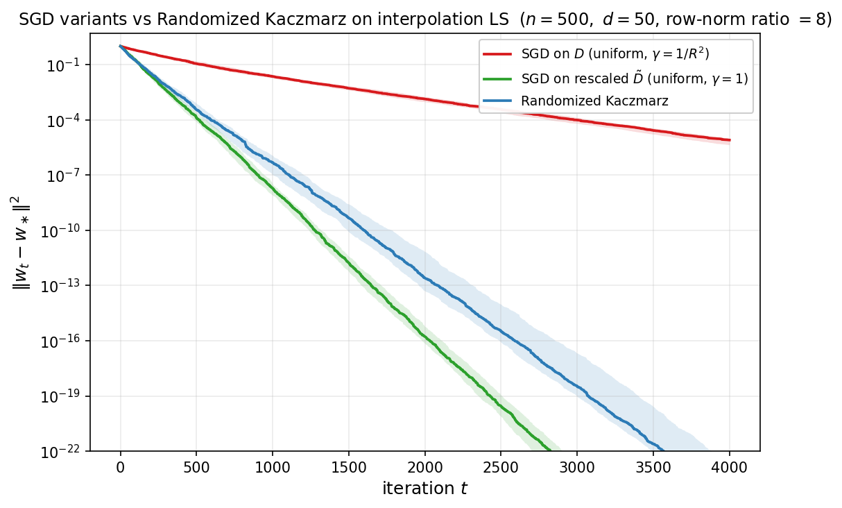
The Kaczmarz method itself, in its deterministic cyclic form, dates back to Kaczmarz [Kac37]. The randomized variant of Algorithm 2 and the geometric rate of Theorem 8.5 are due to Strohmer and Vershynin [SV09]; the connection between Kaczmarz and importance-sampled SGD on interpolation problems was articulated by Needell, Srebro, and Ward [NSW16], and the broader family of randomized iterative methods (block, sketch-and-project, and accelerated variants) is unified by Gower and Richtárik [GR15].
9. Lower Bounds for First-Order and Stochastic Algorithms
This section establishes that the upper bounds developed in Sections 2–4 and Section 8 are sharp, by exhibiting matching lower bounds in two settings of interest. The first is the deterministic optimization setting of Sections 2–4: we close the loophole left by the polynomial/Krylov framework, which only constrains methods whose iterates lie in $x_0 + \mathcal{K}_k(A,r_0)$, and show that even algorithms allowed to query gradients at arbitrary points cannot beat the Chebyshev/CG rate $O(\sqrt{\kappa}\,\log(1/\varepsilon))$. The hard instance is the tridiagonal chain quadratic of Nemirovski and Yudin [NY83]. The second is the stochastic estimation setting of Section 8: we show that on the well-specified additive-Gaussian-noise least-squares problem, no algorithm processing $T$ samples can extract excess risk smaller than $\sigma^2 d/(2T)$, matching tail-averaged streaming SGD up to an absolute constant. The argument is the elegant Bayesian-Gaussian-prior proof of Mourtada [Mou22].
For the first setting, we restrict to deterministic first-order algorithms, by which we mean a procedure $\mathcal{A}$ producing iterates $x_0, x_1, \ldots \in \mathbb{R}^d$ in which $x_0$ is a fixed deterministic vector — depending on the problem only through known parameters— and $x_{t+1}$ is a fixed deterministic function of the past gradients $g_0 = \nabla f(x_0), \ldots, g_t = \nabla f(x_t)$. This includes gradient descent with any sequence of stepsizes, conjugate gradients, and indeed any reasonable first-order method.
Zero-chain quadratics
Write $E_m := \operatorname{span}\lbrace e_1,\dots,e_m\rbrace$ for the span of the first $m$ standard basis vectors of $\mathbb{R}^d$, with the convention $E_0 := \lbrace 0\rbrace$. The structural feature that drives the entire lower-bound argument is the following property of certain convex quadratics, which controls how the support of iterates can grow under first-order queries.
Definition (Zero-chain quadratic). A convex quadratic $\bar f : \mathbb{R}^d \to \mathbb{R}$ is called a zero-chain quadratic if it satisfies the chain property
\[z \in E_m \quad \Longrightarrow \quad \nabla\bar f(z) \in E_{m+1}, \qquad \forall m = 0, 1, \ldots, d-1.\]In words: starting from any vector supported on the first $m$ coordinates, the gradient is supported on the first $m+1$ coordinates. Each gradient query thus advances the support by at most one new coordinate.
Example (Tridiagonal chain quadratic). The canonical example, due to Nemirovski and Yudin, is the quadratic on $\mathbb{R}^d$
\[\bar f(z) \;=\; \tfrac{1}{2}\, z^\top T z - e_1^\top z,\]where $T \in \mathbb{R}^{d\times d}$ is the symmetric tridiagonal matrix
\[T \;=\; \begin{pmatrix} 2 & -1 & 0 & \cdots & 0 \\ -1 & 2 & -1 & \ddots & \vdots \\ 0 & -1 & 2 & \ddots & 0 \\ \vdots & \ddots & \ddots & \ddots & -1 \\ 0 & \cdots & 0 & -1 & 2 \end{pmatrix}.\]The matrix $T$ is positive definite, with eigenvalues $\lambda_j(T) = 4\sin^2\bigl(j\pi/(2(d+1))\bigr)$ for $j=1,\ldots,d$, so $\bar f$ has a unique minimizer. This minimizer solves $T z^\ast = e_1$, and the tridiagonal recursion gives the explicit solution
\[z^\ast_i \;=\; 1 - \frac{i}{d+1}, \qquad i = 1, \ldots, d;\]every coordinate of $z^\ast$ is nonzero, with magnitudes decreasing linearly from near $1$ at $i = 1$ to near $0$ at $i = d$. The chain property is immediate from tridiagonality of $T$: the $i$th entry of $\nabla\bar f(z) = Tz - e_1$ depends only on $z_{i-1}, z_i, z_{i+1}$, so a vector supported on the first $m$ coordinates produces a gradient supported on the first $m+1$. Hence $\bar f$ is a zero-chain quadratic.
The animation below shows the chain property at work: gradient descent is run on $\bar f$ from $x_0 = 0$, and at every step the supports of $x_t$ (left panel) and $\nabla\bar f(x_t)$ (right panel) are exactly ${1,\ldots,t}$ and ${1,\ldots,t+1}$. Untouched coordinates are gray; activated coordinates are blue.
Example (Rescaling). The class of zero-chain quadratics is closed under positive scalar rescaling of the input and output: if $\bar f$ is a zero-chain quadratic on $\mathbb{R}^d$ and $\alpha, \gamma > 0$ are any constants, then the rescaled function
\[f(x) \;:=\; \alpha\,\bar f(\gamma\,x)\]is itself a zero-chain quadratic. Indeed, the chain rule gives $\nabla f(x) = \alpha\gamma\,\nabla\bar f(\gamma x)$ and the zero-chain property follows immediately. This closure under rescaling will let us tune the smoothness constant and the initial distance $\lVert x_0 - x^\ast\rVert$ to any prescribed values without losing the chain structure.
If we had a guarantee that the iterates of any deterministic first-order method always satisfied $x_t \in E_{2t+1}$, the chain property would already yield a clean lower bound on $\lVert x_t - x^\ast\rVert$ from the part of the minimizer that the iterate cannot reach. Of course, no such guarantee holds — a method is free to query off-coordinate points. The next lemma resolves the difficulty: by composing a zero-chain quadratic with a carefully chosen rotation, we force any deterministic first-order method to discover new coordinates two at a time.
The rotation lemma
Lemma 9.1 (Rotation neutralizes arbitrary queries). Let $\bar f$ be a zero-chain quadratic on $\mathbb{R}^d$, fix $k \ge 0$, and assume $d \ge 2k + 2$. For every deterministic first-order algorithm $\mathcal{A}$ there exists an orthogonal matrix $Q \in \mathbb{R}^{d\times d}$ such that, when $\mathcal{A}$ is run on
\[f(x) \;:=\; \bar f(Q^\top x),\]the iterates $x_0, x_1, \ldots, x_k$ produced by $\mathcal{A}$ satisfy
\[Q^\top x_t \in E_{2t+1}, \qquad Q^\top \nabla f(x_t) \in E_{2t+2}, \qquad t = 0, 1, \ldots, k.\]So although $\mathcal{A}$ is allowed to query anywhere in $\mathbb{R}^d$, on the rotated instance its information is forced into the controlled ladder $E_1, E_3, E_5, \ldots$. The proof constructs the columns of $Q$ inductively, exploiting the fact that the algorithm, being deterministic, must commit to its $(t+1)$-st query before seeing how $Q$ is completed past the columns already used.
Proof. Write $Q = [q_1, q_2, \ldots, q_d]$, with the columns $q_i$ to be chosen orthonormal. We construct them two at a time, maintaining the invariant
\[Q^\top x_i \in E_{2i+1}, \qquad Q^\top g_i \in E_{2i+2}, \qquad g_i := \nabla f(x_i),\]for every completed round $i$. The animation below previews the construction: each round adds two new columns of $Q$ (orange strip on the right), the rotated iterate $Q^\top x_t$ acquires two new nonzero coordinates (heatmap column), and the rotated representations of earlier iterates remain frozen — the new $q$’s lie in the orthogonal complement of everything queried so far, so $Q^\top x_s$ for $s < t$ is unaffected by extending $Q$.
Base step ($t = 0$). The algorithm chooses $x_0$ before any gradients are available, so $x_0$ is a fixed deterministic vector. If $x_0 \neq 0$, choose $q_1 = x_0/\lVert x_0\rVert$; if $x_0 = 0$, choose $q_1$ to be any unit vector. In either case $x_0 \in \operatorname{span}\lbrace q_1\rbrace$, and therefore $Q^\top x_0 \in E_1$. Before the gradient oracle can return $g_0 = \nabla f(x_0) = Q\,\nabla\bar f(Q^\top x_0)$, we also commit $q_2$ to be any unit vector orthogonal to $q_1$. With $q_1, q_2$ fixed, the chain rule gives $Q^\top g_0 = \nabla \bar f(Q^\top x_0)$, and the chain property of $\bar f$ yields $Q^\top g_0 \in E_2$.
Inductive step. Suppose the invariant holds for rounds $0, \dots, t$ with $t \le k-1$, and that $q_1, \dots, q_{2t+2}$ have already been fixed. By assumption, $Q^\top x_i \in E_{2i+1}$ and $Q^\top g_i \in E_{2i+2}$ for all $i \le t$, so each of the past oracle answers $g_0, \dots, g_t$ is determined by the columns $q_1,\dots,q_{2t+2}$ alone. How we eventually complete $Q$ on the orthogonal complement of $\operatorname{span}\lbrace q_1,\dots,q_{2t+2}\rbrace$ does not affect any of those answers.
Since $\mathcal{A}$ is deterministic, the next iterate $x_{t+1} = \Phi_{t+1}(g_0, \dots, g_t)$ is a fixed vector of $\mathbb{R}^d$, known to us before any column of $Q$ outside $S_t := \operatorname{span}\lbrace q_1,\dots,q_{2t+2}\rbrace$ is committed. Decompose $x_{t+1}$ into its $S_t$- and $S_t^\perp$-components,
\[x_{t+1} = P_{S_t} x_{t+1} + \underbrace{P_{S_t^{\perp}} x_{t+1}}_{=:r_{t+1}},\]and choose the next basis vector along the orthogonal projection of $x_{t+1}$ onto $S_t^\perp$: if $r_{t+1} \neq 0$, set $q_{2t+3} = r_{t+1}/\lVert r_{t+1}\rVert$; otherwise let $q_{2t+3}$ be any unit vector in $S_t^\perp$. In either case $q_{2t+3} \perp S_t$ and $x_{t+1} \in \operatorname{span}\lbrace q_1,\dots,q_{2t+3}\rbrace$, so $Q^\top x_{t+1} \in E_{2t+3}$.
Next we commit one more column, $q_{2t+4}$, taken to be any unit vector in $S_t^\perp$ orthogonal to $q_{2t+3}$. Such a vector exists because $\dim S_t^\perp = d - (2t+2) \ge 2$ when $t \le k-1$ and $d \ge 2k+2$. With $q_1, \dots, q_{2t+4}$ now committed, the chain rule $\nabla f(x) = Q\,\nabla\bar f(Q^\top x)$ gives $Q^\top g_{t+1} = \nabla\bar f(Q^\top x_{t+1})$. Plugging the containment $Q^\top x_{t+1} \in E_{2t+3}$ into the chain property of $\bar f$ then yields
\[Q^\top g_{t+1} \in E_{2t+4},\]which completes the inductive step. The remaining columns $q_{2k+3}, \dots, q_d$ play no role during the first $k$ rounds and may be completed to an orthonormal basis arbitrarily once the algorithm has terminated. $\square$
Lemma 9.1 is the formal reason that off-Krylov queries do not break worst-case lower bounds. Such queries do break the literal claim that all iterates lie in a Krylov subspace, but on a suitably rotated zero-chain quadratic they still uncover new information only one dimension at a time. The lower-bound recipe is therefore:
- Pick a zero-chain quadratic $\bar f$, possibly after rescaling.
- Use Lemma 9.1 to reduce any deterministic first-order method on a rotated instance to a zero-respecting method on $\bar f$ — one whose iterates lie in the growing chain of coordinate subspaces $E_1 \subseteq E_3 \subseteq E_5 \subseteq \cdots$.
- Lower-bound the error of any point supported on only the first $2k+1$ coordinates.
Step 3 is now an explicit calculation on the tridiagonal example.
The lower bound
Theorem 9.2 (Lower bound). Fix $k \ge 1$ and $\beta, R > 0$, and set $d := 4k+2$. There exist a convex quadratic $f : \mathbb{R}^d \to \mathbb{R}$ with $\lVert\nabla^2 f\rVert_{\mathrm{op}} \le \beta$ and an initialization $x_0$ with $\lVert x_0 - x^\ast\rVert = R$ such that for every deterministic first-order algorithm $\mathcal{A}$ the iterates satisfy
\[f(x_k) - f^\ast \;\ge\; \frac{3}{128}\cdot\frac{\beta\,R^2}{(k+1)^2}.\]Proof. Set $d := 4k+2$ and let $\bar f(z) = \tfrac12 z^\top T z - z^\top e_1$ be the tridiagonal chain quadratic on $\mathbb{R}^d$, with $T$ the tridiagonal Hessian and $z^\ast$ its minimizer. Fix the rescalings
\[\alpha \;:=\; \frac{\beta\,R^2}{\lVert T\rVert_{\mathrm{op}}\,\lVert z^\ast\rVert^2}, \qquad \gamma \;:=\; \frac{\lVert z^\ast\rVert}{R}.\]By the rescaling example, $\tilde f(z) := \alpha\,\bar f(\gamma\,z)$ is itself a zero-chain quadratic. Lemma 9.1 applied to $\tilde f$ therefore furnishes an orthogonal $Q$ such that, when $\mathcal{A}$ is run from $x_0 = 0$ on the hard instance
\[f(x) \;:=\; \tilde f(Q^\top x) \;=\; \alpha\,\bar f\bigl(\gamma\,Q^\top x\bigr),\]the iterates satisfy
\[Q^\top x_t \;\in\; E_{2t+1}, \qquad \forall\, t = 0, 1, \ldots, k.\]This function $f$ has the required parameters: its Hessian is $\alpha\gamma^2\,Q T Q^\top$, so $\lVert\nabla^2 f\rVert_{\mathrm{op}} = \alpha\gamma^2\,\lVert T\rVert_{\mathrm{op}} = \beta$, and its minimizer is $x^\ast = Q\,z^\ast/\gamma$ with $\lVert x_0 - x^\ast\rVert = \lVert z^\ast\rVert/\gamma = R$.
Setting $w := \gamma\,Q^\top x_k \in E_{2k+1}$, we obtain
\[f(x_k) - f^\ast \;=\; \alpha\,\bigl(\bar f(w) - \bar f^\ast\bigr) \;\ge\; \alpha\,\bigl(\,\textstyle\min_{u \in E_{2k+1}}\,\bar f(u)\, -\, \bar f^\ast\bigr).\]The minimizer of $\bar f$ over $E_{2k+1}$ solves the truncated tridiagonal system $T_{2k+1}\,u_{1:2k+1} = e_1$, with explicit solution
\[u_i = 1 - \frac{i}{2k+2} \qquad\forall i \le 2k+1,\]and $u_i = 0$ otherwise. Since any minimizer of $y$ of a truncated chain satisfies $T_m\,y_{1:m} = e_1$, plugging this expression into $\bar f$ directly shows $\bar f(y) = -\tfrac{1}{2}\,y_1$. Therefore we deduce
\[\min_{u \in E_{2k+1}} \bar f(u) - \bar f^\ast \;=\; \frac{1}{2}\!\left[\frac{d}{d+1} - \frac{2k+1}{2k+2}\right] \;=\; \frac{d - 2k - 1}{2\,(d+1)(2k+2)} \;=\; \frac{2k+1}{2\,(4k+3)(2k+2)}.\]The elementary bounds $\lVert T\rVert_{\mathrm{op}} \le 4$ and
\[\lVert z^\ast\rVert^2 \;=\; \frac{1}{(d+1)^2}\sum_{i=1}^d i^2 \;=\; \frac{d(2d+1)}{6(d+1)} \;\le\; \frac{d}{3} \;=\; \frac{4k+2}{3}\]yield $\alpha \ge 3\,\beta R^2 / (4(4k+2))$. Substituting gives
\[f(x_k) - f^\ast \;\ge\; \frac{3\,\beta R^2}{4(4k+2)} \cdot \frac{2k+1}{2(4k+3)(2k+2)} \;=\; \frac{3\,\beta R^2}{32\,(4k+3)\,(k+1)} \;\ge\; \frac{3}{128}\cdot\frac{\beta R^2}{(k+1)^2},\]as claimed. $\square$
The bound matches the upper bound $\beta R^2/(8k^2)$ of Theorem 6.2 up to an absolute constant: the $O(\sqrt{\beta R^2/\varepsilon})$ iteration complexity of Chebyshev acceleration and conjugate gradients in the smooth convex regime is therefore optimal among deterministic first-order methods on quadratics, even allowing arbitrary off-Krylov queries.
The hard quadratic and the rotation argument are due to Nemirovski and Yudin [NY83]; modern treatments appear in Nesterov [Nes04, Nes18]. The same chain construction underlies the corresponding lower bounds for general smooth strongly convex and smooth convex minimization beyond the quadratic class, with only minor adjustments to the choice of $T$ and the way the chain quadratic is embedded in $\mathbb{R}^d$.
Lower bounds with structured spectrum
Theorem 9.2 closes the gap in the worst case: no deterministic first-order method beats Chebyshev/CG on every quadratic with $\lVert\nabla^2 f\rVert_{\mathrm{op}} \le \beta$. Recall, however, that Section 7 showed that structured spectra — power-law densities $\phi(\lambda) = M\lambda^{a-1}$ and Marchenko–Pastur laws, for instance — yield much faster CG rates than the worst case allows. A natural question is whether these structured rates are themselves tight against arbitrary deterministic first-order methods.
The answer is that the structured rate is tight: the same residual polynomial that drives the CG upper bound also certifies a matching lower bound for every deterministic first-order method, up to a constant shift $k \mapsto 2k+1$. Our goal is to show why this is the case.
We begin by recalling from Section 7 the spectral measure $\mu := \sum_{i=1}^d c_i^2\,\delta_{\lambda_i}$ on $[0,\beta]$, where $c_i$ are the coordinates of the initial error $x_0 - x^\ast$ in the eigenbasis of $A$. Rewriting $(4b)$ as an integral against $\mu$ gives the spectral-measure form of the CG identity:
\[f(x_k^{\mathrm{CG}}) - f^\ast \;=\; \tfrac{1}{2}\min_{\substack{p \in \mathcal{P}_k \\ p(0) = 1}}~\int_0^\beta \lambda\,p(\lambda)^2\,d\mu(\lambda), \tag{61}\]We will now show that the conjugate gradient method is optimal in a much stronger sense than the minimax bound we have already proved: the worst-case instance for any deterministic first-order algorithm can be chosen to have any prescribed spectral measure.
We will need the following simple helper lemma. We call a tridiagonal matrix $A\in\mathbb{R}^{d\times d}$ irreducible if all of its off-diagonal entries are nonzero:
\[A_{i,i+1} = A_{i+1,i} \ne 0, \qquad \forall\, i = 1, \ldots, d-1.\]Lemma 9.3 (Krylov subspaces of irreducible tridiagonal matrices). If $A \in \mathbb{R}^{d \times d}$ is irreducible and tridiagonal, then the Krylov subspace $\mathcal{K}_t(A, e_1)$ coincides with the coordinate subspace $E_t$ for every $t \ge 1$.
Proof. Since $A$ is tridiagonal, the inclusion $A E_m \subset E_{m+1}$ holds, and therefore
\[\operatorname{span}\{e_1,\, Ae_1,\, \ldots,\, A^{m-1} e_1\} \subset E_m. \tag{62}\]Conversely, the $(j+1)$-st coordinate of $A^j e_1$ is
\[A_{j+1,j}\,A_{j,j-1}\cdots A_{2,1},\]which is nonzero by irreducibility. Thus we have $A^j e_1 \in E_{j+1} \setminus E_j$, and by dimension counting the inclusion $(62)$ holds as equality. $\square$
Next, we need the following lemma that constructs an irreducible, positive semidefinite, tridiagonal problem with any prescribed spectral measure.
Lemma 9.4 (Exact Jacobi realization of a finite measure). Consider an atomic measure $\mu = \sum_{i=1}^d w_i\,\delta_{\theta_i}$ with atoms $0 < \theta_1 < \cdots < \theta_d \le \beta$ and weights $w_i > 0$. Then there exist an irreducible, positive-semidefinite, tridiagonal matrix $A \in \mathbb{R}^{d \times d}$ with $\lVert A\rVert_{\mathrm{op}} \le \beta$ and a scalar $\tau > 0$ such that the spectral measure $\mu_{A,x^\ast}$ of the convex quadratic problem with data
\[x_0 = 0, \qquad b := \tau e_1, \qquad x^\ast := A^{-1} b,\]coincides exactly with $\mu$.
Proof. Set $M_2 := \int \lambda^2\,d\mu$ and define
\[d\nu \;:=\; \frac{\lambda^2}{M_2}\,d\mu.\]Then $\nu$ is a probability measure supported on the same $d$ atoms as $\mu$. The space $L^2(\nu)$ is simply the $d$-dimensional space of functions on these atoms, and the monomials $1, \lambda, \ldots, \lambda^{d-1}$ span it. Applying Gram–Schmidt to these monomials, we obtain an orthonormal basis
\[q_0 \equiv 1,\; q_1,\; \ldots,\; q_{d-1},\]where $q_i$ has degree exactly $i$ and is orthogonal to every polynomial of degree at most $i-1$.
Let $M_\lambda$ be the operator of multiplication by $\lambda$ on $L^2(\nu)$, and let $A$ be its matrix in the basis ${q_0, \ldots, q_{d-1}}$, that is:
\[A_{ij} \;:=\; \langle q_{i-1},\, \lambda\,q_{j-1}\rangle_{L^2(\nu)}, \qquad i,j = 1, \ldots, d.\]The matrix $A$ is symmetric. It is also tridiagonal: if $i > j+1$, then $\lambda\,q_{j-1}$ has degree $j \le i-2$ and is therefore orthogonal to $q_{i-1}$. Symmetry gives the same conclusion when $i < j-1$.
We next show that $A$ is irreducible. Choose each $q_n$ to have positive leading coefficient $\kappa_n > 0$. Comparing leading terms in the expansion of $\lambda\,q_n$ in the orthonormal basis gives
\[\lambda\,q_n \;=\; \frac{\kappa_n}{\kappa_{n+1}}\,q_{n+1} + \text{lower-degree terms}.\]Taking inner products with $q_{n+1}$, we get
\[A_{n+2,n+1} \;=\; \langle q_{n+1},\, \lambda\,q_n\rangle_{L^2(\nu)} \;=\; \frac{\kappa_n}{\kappa_{n+1}} \;>\; 0.\]Thus every off-diagonal entry of $A$ is nonzero.
The spectral bounds are immediate from the multiplication operator. If $p \in L^2(\nu)$ is nonzero, then
\[\langle p,\, M_\lambda\,p\rangle_{L^2(\nu)} \;=\; \int \lambda\,p(\lambda)^2\,d\nu(\lambda) \;>\; 0,\]and, since $\nu$ is supported on $(0, \beta]$,
\[\langle p,\, M_\lambda\,p\rangle_{L^2(\nu)} \;\le\; \beta\,\lVert p\rVert_{L^2(\nu)}^2.\]Hence $A$ is positive definite and $\lVert A\rVert_{\mathrm{op}} \le \beta$.
It remains to identify the spectral measure. For any vector $z$ and any polynomial $p$, the spectral measure of $z$ satisfies
\[z^\top p(A)\,z \;=\; \int p(\lambda)\,d\mu_{A,z}(\lambda); \tag{63}\]this is immediate from an eigenvalue decomposition of $A$. Set $\tau := \sqrt{M_2}$, $b := \tau\,e_1$, and
\[x^\ast \;:=\; A^{-1} b \;=\; \tau\,A^{-1} e_1.\]The vector $e_1$ corresponds to the constant polynomial $q_0 \equiv 1$, and $A$ represents multiplication by $\lambda$. Therefore, for every polynomial $p$, we have
\[\begin{aligned} (x^\ast)^\top p(A)\,x^\ast &= \tau^2\,e_1^\top A^{-1} p(A)\,A^{-1} e_1 \\ &= \tau^2\,\langle 1,\, \lambda^{-1}\,p(\lambda)\,\lambda^{-1}\rangle_{L^2(\nu)} \\ &= \tau^2 \int \lambda^{-2}\,p(\lambda)\,d\nu(\lambda) \\ &= \int p(\lambda)\,d\mu(\lambda). \end{aligned}\]Combining this identity with $(63)$ shows that $\mu_{A,x^\ast}$ and $\mu$ integrate every polynomial in the same way. Since both measures are finite atomic, they are equal. $\square$
We are now ready to prove the optimality of CG. To simplify notation, for a positive measure $\nu$ on $(0,\beta]$, define
\[\mathcal{E}_t(\nu) \;:=\; \tfrac{1}{2}\min_{\substack{p \in \mathcal{P}_t \\ p(0)=1}}\int_0^\beta \lambda\,p(\lambda)^2\,d\nu(\lambda).\]Theorem 9.5 (Optimality of CG). Fix an iteration counter $t \ge 0$, a constant $\beta > 0$, and a finite positive atomic measure $\mu$ on $(0,\beta]$ that has at least $2t+2$ atoms. Then for every deterministic first-order algorithm there exists a convex quadratic problem instance whose spectral error measure $\mu_{A,x^\ast}$ is exactly $\mu$ and whose $t$-th iterate after initialization $x_0 = 0$ satisfies
\[f(x_t) - f^\ast \;\ge\; \mathcal{E}_{2t+1}(\mu).\]Proof. Fix a deterministic first-order algorithm $\mathcal{A}$, and write
\[\mu \;=\; \sum_{i=1}^d w_i\,\delta_{\lambda_i}, \qquad 0 < \lambda_1 < \cdots < \lambda_d \le \beta, \qquad w_i > 0,\]where $d \ge 2t + 2$. Applying Lemma 9.4 to $\mu$, we obtain an irreducible, tridiagonal, positive semidefinite matrix $A$ with $\lVert A\rVert_{\mathrm{op}} \le \beta$, a scalar $\tau > 0$, and the vector $b = \tau e_1$ such that the quadratic
\[\bar f(z) \;=\; \tfrac{1}{2} z^\top A z - b^\top z\]has minimizer $x^\ast = A^{-1}b$ and spectral error measure $\mu_{A,x^\ast} = \mu$.
Moreover $\bar f$ is zero-chain, since tridiagonality gives $A E_m \subset E_{m+1}$ and $b \in E_1$. Applying Lemma 9.1, we deduce that there is an orthogonal matrix $Q$ such that the algorithm $\mathcal{A}$ applied to
\[f(x) \;=\; \bar f(Q^\top x)\]produces iterates satisfying
\[Q^\top x_s \in E_{2s+1}, \qquad \forall\, s = 0, 1, \ldots, t.\]Orthogonal changes of variables preserve the spectral error measure, and therefore the rotated instance $f$ also has spectral error measure $\mu$. Since $2t+1 \le d$ and $b$ is a nonzero multiple of $e_1$, the helper lemma above ensures the equality
\[E_{2t+1} \;=\; \mathcal{K}_{2t+1}(A, b).\]Thus the inclusion $Q^\top x_t \in \mathcal{K}_{2t+1}(A, b)$ holds, and consequently
\[f(x_t) - f^\ast \;=\; \bar f(Q^\top x_t) - \bar f^\ast \;\ge\; \min_{u \,\in\, \mathcal{K}_{2t+1}(A,b)} \bar f(u) - \bar f^\ast.\]Using the Krylov polynomial identity $(61)$ and the equality $\mu_{A,x^\ast} = \mu$, the right-hand side equals $\mathcal{E}_{2t+1}(\mu)$, which completes the proof. $\square$
Let us spell out what the construction gives in two common spectral regimes.
Example (Atomic power laws). For $a > -1$ and $d \ge 2t + 2$, set
\[\mu_d \;=\; \sum_{i=1}^d w_i\,\delta_{\lambda_i}, \qquad \lambda_i \asymp \frac{i}{d}, \qquad w_i \asymp d^{-a}\,i^{a-1}.\]Theorem 9.5 gives the lower bound $\mathcal{E}_{2t+1}(\mu_d)$. For $d$ large relative to $t$, the atomic measure $\mu_d$ is a Riemann discretization of the continuum power-law density $\phi(\lambda) = \lambda^{a-1}$ on $(0,1]$, so
\[\mathcal{E}_{2t+1}(\mu_d) \;\asymp\; \min_{\substack{p \in \mathcal{P}_t \\ p(0)=1}}\; \int \lambda\,p(\lambda)^2\,\lambda^{a-1}\,d\lambda \;\asymp\; t^{-2(a+1)}.\]This is exactly the rate established for CG under a power-law spectral density in Theorem 7.6. Thus the lower bound scales as $t^{-2(a+1)}$, matching the CG upper bound up to the universal $k \leftrightarrow 2k+1$ degree shift.
Example (Atomic Marchenko–Pastur hard edge). For $d \ge 2t + 2$, set
\[\mu_d \;=\; \sum_{i=1}^d w_i\,\delta_{\lambda_i}, \qquad \lambda_i \asymp \left(\frac{i}{d}\right)^{\!2}, \qquad w_i \asymp d^{-1}.\]Then $\mu_d([0, s]) \asymp s^{1/2}$, so the continuum hard-edge limit is the power-law case $a = 1/2$. For $d$ large relative to $t$,
\[\mathcal{E}_{2t+1}(\mu_d) \;\asymp\; \min_{\substack{p \in \mathcal{P}_t \\ p(0)=1}}\; \int \lambda\,p(\lambda)^2\,\lambda^{-1/2}\,d\lambda \;\asymp\; t^{-3}.\]This is the $a = 1/2$ specialization of the previous example via Theorem 7.6, and matches the $k^{-3}$ Marchenko–Pastur CG rate established in Theorem 7.5. Thus the lower bound scales as $t^{-3}$.
Theorem 9.5 is stated for finite atomic measures, but the natural spectral models in Section 7 — power-law densities and the Marchenko–Pastur law — are continuous. We now show that this distinction is irrelevant for any fixed iteration counter $t$: for any prescribed positive measure $\mu$ on $(0,\beta]$ and any deterministic first-order algorithm, there is a hard instance in $\mathbb{R}^{2t+2}$ matching the lower bound from Theorem 9.5, with a spectral measure that is indistinguishable from $\mu$ when tested against polynomials of degree at most $4t+3$. This is the content of Theorem 9.7 below.
The construction relies on a classical ingredient: Gauss quadrature. This basic technique, summarized in Lemma 9.6, shows that for any nondegenerate measure $\mu$ on a compact interval, there exists a measure $\mu_N$ supported only on $N$ points, such that every polynomial of degree at most $2N-1$ integrates to the same quantity with respect to both $\mu$ and $\mu_N$. In this way, we can reduce a general measure $\mu$ to an atomic measure $\mu_N$ supported on $N \approx t$ points, to which Theorem 9.5 then applies.
Lemma 9.6 (Gauss quadrature). Let $\mu$ be a positive Borel measure on $[0,\beta]$ supported on at least $N+1$ distinct points, with finite moments up to order $2N-1$. Then there exist points $\theta_1 < \cdots < \theta_N$ in the interior of the convex hull of $\mathrm{supp}(\mu)$ and positive weights $w_1,\ldots,w_N > 0$ such that the atomic measure
\[\mu_N \;:=\; \sum_{j=1}^N w_j\,\delta_{\theta_j} \tag{64}\]agrees with $\mu$ on every polynomial of degree at most $2N-1$:
\[\int P\,d\mu_N \;=\; \int P\,d\mu \qquad \text{for every } P \in \mathcal{P}_{2N-1}. \tag{$\dagger$}\]The measure $\mu_N$ is called the $N$-point Gauss quadrature rule for $\mu$. Figure 9.1 illustrates the rule for a Beta-like density: just $N=5$ atoms suffice to reproduce the continuous integral exactly on every polynomial of degree at most $2N-1 = 9$.
![Gauss quadrature for a non-uniform measure on $[0,1]$: left, the continuous density (blue) and the $N=5$ atoms of $\mu_N$ (red stems with heights proportional to the weights $w_j$); right, a test polynomial $P \in \mathcal{P}_9$ together with its values at the Gauss nodes — the continuous integral $\int P\,d\mu$ equals the discrete sum $\sum_j w_j\,P(\theta_j)$ exactly.](/DSC-243/figures/gauss_quadrature.png)
Proof. We will choose the nodes first, then choose the weights so that all lower-degree polynomials are integrated correctly.
Apply Gram–Schmidt in $L^2(\mu)$ to the monomials ${1,\lambda,\ldots,\lambda^N}$, producing orthonormal polynomials $\tilde p_0,\ldots,\tilde p_N$ with $\deg \tilde p_n=n$. This construction is well-defined: after subtracting the projection of $\lambda^n$ onto the lower-degree polynomials, the remaining polynomial cannot have zero $L^2(\mu)$ norm unless it vanishes on $\mathrm{supp}(\mu)$; but a nonzero polynomial of degree at most $n\le N$ cannot vanish on the at least $N+1$ distinct support points of $\mu$. Take the quadrature nodes $\theta_1<\cdots<\theta_N$ to be the roots of $\tilde p_N$.
We claim that these roots are real, simple, and lie in the interior of the convex hull of $\mathrm{supp}(\mu)$. The key point is that $\tilde p_N$ must change sign at least $N$ times across the support of $\mu$. To see this, suppose instead that it changes sign only $m<N$ times. Let $\xi_1<\cdots<\xi_m$ denote the corresponding sign-change locations. Between consecutive $\xi_i$’s, the sign of $\tilde p_N$ is constant, and crossing a $\xi_i$ flips the sign. Hence the polynomial
\[r(\lambda):=\prod_{i=1}^m(\lambda-\xi_i)\]changes sign at exactly the same locations. After multiplying $r$ by $-1$ if necessary, we therefore have $\tilde p_N(\lambda)\,r(\lambda)\ge 0$ for every $\lambda\in \mathrm{supp}(\mu)$. Moreover, the product is not identically zero on $\mathrm{supp}(\mu)$: otherwise $\tilde p_N$ would vanish on all of $\mathrm{supp}(\mu)$ except possibly the $m$ points $\xi_i$, forcing the degree-$N$ polynomial $\tilde p_N$ to have too many zeros. Since we have $r\in \mathcal{P}_m\subseteq \mathcal{P}_{N-1}$, we get
\[\int \tilde p_N(\lambda)\,r(\lambda)\,d\mu(\lambda)>0,\]contradicting the orthogonality $\tilde p_N \perp \mathcal{P}_{N-1}$.
Thus $\tilde p_N$ has at least $N$ sign changes on the support. Each sign change gives a distinct real zero, while $\deg \tilde p_N=N$, so these are exactly the $N$ distinct roots of $\tilde p_N$. The roots lie between support points, hence in the interior of the convex hull of $\mathrm{supp}(\mu)$.
Now let $\ell_j$ be the polynomial:
\[\ell_j(\lambda):=\prod_{i\ne j}\frac{\lambda-\theta_i}{\theta_j-\theta_i} \qquad\textrm{and note}\qquad \ell_j(\theta_i)=\mathbf{1}_{i=j},\]Define the weights
\[w_j:=\int \ell_j(\lambda)\,d\mu(\lambda).\]We claim that these weights give exact integration on $\mathcal{P}_{2N-1}$. Fix $P\in \mathcal{P}_{2N-1}$. Since $\tilde p_N$ is a degree-$N$ polynomial, ordinary polynomial long division lets us write $P$ uniquely as
\[P = \tilde p_N\,s + r, \qquad \deg(s),\,\deg(r) \le N-1.\]Here $s$ is the quotient and $r$ is the remainder. This decomposition is useful because the quotient term $\tilde p_N\,s$ contributes nothing to either side of the desired identity. Against $\mu$, it integrates to zero by orthogonality, since $s\in\mathcal{P}_{N-1}$ and $\tilde p_N$ is orthogonal to $\mathcal{P}_{N-1}$. Against $\mu_N$, it also integrates to zero because $\mu_N$ is supported exactly on the roots $\theta_j$ of $\tilde p_N$. Therefore, to prove exactness for $P$, it remains only to prove exactness for the lower-degree remainder $r\in\mathcal{P}_{N-1}$.
Now use the fact that a polynomial of degree at most $N-1$ is completely determined by its values at $N$ distinct points. The Lagrange polynomials $\ell_1,\ldots,\ell_N$ were built precisely for this purpose: $\ell_j(\theta_i)=\mathbf{1}_{i=j}$, so the linear combination
\[\sum_{j=1}^N r(\theta_j)\,\ell_j.\]has the same value as $r$ at every node $\theta_i$. Since both sides have degree at most $N-1$, equality at the $N$ distinct nodes forces equality $r=\sum_{j=1}^N r(\theta_j)\,\ell_j$ as polynomials. Therefore
\[\int r\,d\mu =\sum_{j=1}^N r(\theta_j)\int \ell_j\,d\mu =\sum_{j=1}^N r(\theta_j)w_j =\int r\,d\mu_N.\]This proves exactness for the remainder. It remains only to check that the weights are positive. The polynomial $\ell_j-\ell_j^2$ vanishes at every node $\theta_i$, so it is divisible by $\tilde p_N$:
\[\ell_j-\ell_j^2=\tilde p_N\,h_j\]for some $h_j\in\mathcal{P}_{N-2}$. Orthogonality again gives $\int \tilde p_N h_j\,d\mu=0$, and therefore
\[w_j=\int \ell_j\,d\mu=\int \ell_j^2\,d\mu>0.\]Combining this with the reduction from $P$ to $r$ proves $(\dagger)$. $\square$
Combining the Gauss quadrature reduction of Lemma 9.6 with the atomic optimality result of Theorem 9.5 immediately delivers the general lower bound promised at the start of this subsection.
Theorem 9.7 (Optimality of CG up to low-degree moments). Fix an iteration counter $t \ge 0$, a constant $\beta > 0$, and a positive Borel measure $\mu$ on $(0,\beta]$ supported on at least $2t+3$ distinct points. Then for every deterministic first-order algorithm there exists a convex quadratic problem instance on $\mathbb{R}^{2t+2}$ whose spectral error measure $\mu_{A,x^\ast}$ agrees with $\mu$ on $\mathcal{P}_{4t+3}$ and whose $t$-th iterate after initialization $x_0 = 0$ satisfies
\[f(x_t) - f^\ast \;\ge\; \mathcal{E}_{2t+1}(\mu).\]Proof. Fix a deterministic first-order algorithm and set $N := 2t + 2$. By Lemma 9.6, the $N$-point Gauss quadrature rule
\[\mu_N \;=\; \sum_{j=1}^N w_j\,\delta_{\theta_j}, \qquad 0 < \theta_1 < \cdots < \theta_N \le \beta, \qquad w_j > 0,\]agrees with $\mu$ on $\mathcal{P}_{2N-1} = \mathcal{P}_{4t+3}$. Applying Theorem 9.5 to $\mu_N$, we obtain a convex quadratic instance on $\mathbb{R}^N$ whose spectral error measure equals $\mu_N$ exactly and whose $t$-th iterate satisfies
\[f(x_t) - f^\ast \;\ge\; \mathcal{E}_{2t+1}(\mu_N).\]For every $p \in \mathcal{P}_{2t+1}$, the integrand $\lambda\,p(\lambda)^2$ has degree at most $4t+3$, so the moment-matching identity gives $\mathcal{E}_{2t+1}(\mu_N) = \mathcal{E}_{2t+1}(\mu)$, completing the proof. $\square$
A statistical lower bound for stochastic algorithms
We now turn from optimization on a fixed deterministic objective to estimation from noisy stochastic samples. The setting is the streaming least-squares problem of Section 8 specialized to the well-specified additive Gaussian noise model
\[y \;=\; \langle w_\ast, x\rangle + \eta, \qquad \eta \sim \mathcal{N}(0,\sigma^2)\ \text{independent of}\ x.\]In this regime $\Sigma = \sigma^2 H$ gives $\sigma_{\mathrm{MLE}}^2 = \tfrac12 d\sigma^2$ and $\rho_{\mathrm{misspec}} = 1$, and the variance bound of Theorem 8.2 (after a burn-in long enough to eliminate the bias and at $\gamma R^2 = \tfrac12$) reduces to $4d\sigma^2/(T-t)$. We show that this $d\sigma^2/T$ scaling is sharp: no algorithm processing $T$ stochastic samples can achieve lower variance. Tail-averaged constant-stepsize SGD is therefore minimax-optimal on the well-specified least-squares problem.
The argument is short and elegant, and adapts Mourtada’s [Mou22] fixed-design proof to the streaming setting. Recall that the population least-squares risk is
\[L(w) \;:=\; \tfrac{1}{2}\,\mathbb{E}_{(x,y)}\!\left[(y - \langle w, x\rangle)^2\right],\]minimized at $w_\ast$, and the excess risk decomposes as $L(w) - L(w_\ast) = \tfrac{1}{2}\,\lVert w - w_\ast\rVert_H^2$, where $H := \mathbb{E}[x x^\top]$ is the feature covariance.
We will also use the following elementary fact from Bayesian estimation.
Lemma 9.8 (Bayes estimator). Let $(w, z)$ be a pair of random vectors with $z$ observed and $w$ unknown, and fix a matrix $M \succeq 0$. Among all measurable estimators $a(z)$, the quantity
\[\mathbb{E}\,\lVert a(z) - w\rVert_M^2\]is minimized by the conditional expectation $a(z) = \mathbb{E}[w \mid z]$. Moreover, if for each $z$ the conditional density $w \mapsto p(w \mid z)$ is Gaussian, then $\mathbb{E}[w \mid z]$ coincides with the unique maximizer of $w \mapsto p(w \mid z)$.
Proof. Write $m(z) := \mathbb{E}[w \mid z]$. Conditioning on $z$ and expanding the squared $M$-norm gives
\[\begin{aligned} \mathbb{E}\!\left[\lVert a(z)-w\rVert_M^2 \mid z\right] &= \lVert a(z)-m(z)\rVert_M^2 \\ &\qquad + \mathbb{E}\!\left[\lVert m(z)-w\rVert_M^2 \mid z\right], \end{aligned}\]since the cross term has conditional expectation zero. The second term does not depend on $a$, so the first term is minimized by $a(z)=m(z)$. The second claim follows since a Gaussian density is symmetric about its mean, so when $p(\cdot \mid z)$ is Gaussian its unique maximizer is $\mathbb{E}[w \mid z]$. $\square$
Theorem 9.9 (Minimax lower bound for streaming least squares). *Fix $T \ge 1$, a noise level $\sigma > 0$, and a distribution on $\mathbb{R}^d$ with positive-definite covariance $H = \mathbb{E}[x x^\top]$. Suppose the well-specified Gaussian-noise model $y = \langle w_\ast, x\rangle + \eta$ with $\eta \sim \mathcal{N}(0, \sigma^2)$ independent of $x$. Then given $T$ iid samples $(x_1, y_1), \ldots, (x_T, y_T)$ and any (possibly randomized) measurable estimator $\hat w = \hat w(x_1, y_1, \ldots, x_T, y_T)$, there exists $w_{\ast}$ satisfying
\[\mathbb{E}\bigl[L(\hat w) - L(w_\ast)\bigr] \;\ge\; \frac{\sigma^2 d}{2T}.\]Proof. By the excess-risk identity, $L(\hat w) - L(w_\ast) = \tfrac{1}{2}\,\lVert \hat w - w_\ast\rVert_H^2$, so it suffices to lower bound
\[\sup_{w_\ast}\,\mathbb{E}\,\lVert \hat w - w_\ast\rVert_H^2.\]The supremum over $w_\ast$ is bounded below by the expected error under any prior on $w_\ast$. We choose the Gaussian prior $w_\ast \sim \mathcal{N}\bigl(0, \tfrac{\sigma^2}{T\lambda}\,I_d\bigr)$, with $\lambda > 0$ to be sent to zero at the end of the proof. Stack the samples into the data matrix $X \in \mathbb{R}^{T \times d}$ whose $i$-th row is $x_i^\top$, write $\hat H := \tfrac{1}{T}\,X^\top X$ for the empirical covariance, and set $y := X\,w_\ast + \eta$ with $\eta \sim \mathcal{N}(0, \sigma^2 I_T)$ independent of both $w_\ast$ and $X$.
Identifying the Bayes estimator. Set $m(X,y) := \mathbb{E}[w_\ast \mid X, y]$. By Lemma 9.8 applied to the random pair $\bigl(w_\ast,\,(X,y)\bigr)$ with weighting matrix $H$, every estimator $\hat w(X,y)$ satisfies $\mathbb{E}\,\lVert \hat w - w_\ast\rVert_H^2 \ge \mathbb{E}\,\lVert m(X,y) - w_\ast\rVert_H^2$. The conditional density of $w_\ast$ given $(X,y)$ is Gaussian (by Bayes’ rule), so Lemma 9.8 also identifies $m(X,y)$ as the maximizer over $w_\ast$ of $p(w_\ast \mid X, y)$. By Bayes’ rule, $p(w_\ast \mid X, y) \propto p(y \mid w_\ast, X)\,p(w_\ast)$ as a function of $w_\ast$ (the constant of proportionality $p(y \mid X)$ does not depend on $w_\ast$), and inserting the Gaussian densities $y \mid w_\ast, X \sim \mathcal{N}(X w_\ast, \sigma^2 I_T)$ and $w_\ast \sim \mathcal{N}(0, \tfrac{\sigma^2}{T\lambda} I_d)$ gives, on a log scale,
\[\log p(w_\ast \mid X, y) \;=\; -\frac{1}{2\sigma^2}\,\lVert y - X\,w_\ast\rVert^2 \;-\; \frac{T\lambda}{2\sigma^2}\,\lVert w_\ast\rVert^2 \;+\; \text{const},\]where the constant collects all terms independent of $w_\ast$.
Equivalently, $m(X,y)$ minimizes the ridge cost $\lVert y - X w\rVert^2 + T\lambda\,\lVert w\rVert^2$. Differentiating in $w$ and setting the derivative to zero yields the expression
\[m(X, y) \;=\; (X^\top X + T\lambda I)^{-1}\,X^\top y \;=\; \tfrac{1}{T}\,(\hat H + \lambda I)^{-1}\,X^\top y.\]Computing the Bayes risk. Substituting $y = X\,w_\ast + \eta$ and using the identity $(X^\top X + T\lambda I)^{-1}\,X^\top X - I = -T\lambda\,(X^\top X + T\lambda I)^{-1}$ gives the bias–variance decomposition
\[m(X, y) - w_\ast \;=\; -\lambda\,(\hat H + \lambda I)^{-1}\,w_\ast \;+\; \tfrac{1}{T}\,(\hat H + \lambda I)^{-1}\,X^\top \eta.\]We now take the $H$-norm of both sides. Independence of $w_\ast$, $\eta$, and $X$ kills the cross term in $\lVert\,\cdot\,\rVert_H^2$. Computing the two diagonal contributions with $\mathbb{E}[w_\ast w_\ast^\top] = \tfrac{\sigma^2}{T\lambda}\,I$ and $\mathbb{E}[\eta\eta^\top] = \sigma^2 I_T$ yields, after the factorization $\lambda H + H^2 = H(\lambda I + H)$, the estimate
\[\mathbb{E}_{w_\ast, \eta \mid X}\,\lVert m(X, y) - w_\ast\rVert_H^2 \;=\; \frac{\sigma^2}{T}\,\mathrm{Tr}\!\bigl[(\hat H + \lambda I)^{-1}\, H\bigr].\]Averaging over $X$. Operator convexity of $M \mapsto M^{-1}$ on $\mathbb{S}^d_{++}$, applied to the random PSD matrix $\hat H + \lambda I$ with mean $H + \lambda I$, gives the operator Jensen inequality
\[\mathbb{E}_X\!\bigl[(\hat H + \lambda I)^{-1}\bigr] \;\succeq\; (H + \lambda I)^{-1}.\]Taking the trace against $H \succ 0$ and letting $\lambda \downarrow 0$ yields
\[\mathbb{E}_X\,\mathrm{Tr}\!\bigl[(\hat H + \lambda I)^{-1}\, H\bigr] \;\ge\; \mathrm{Tr}\!\bigl[(H + \lambda I)^{-1}\, H\bigr] \;\xrightarrow{\lambda \downarrow 0}\; \mathrm{Tr}\!\bigl[H^{-1}\, H\bigr] \;=\; d.\]Inserting the factor of $\tfrac{1}{2}$ from the excess-risk identity completes the proof. $\square$
The matching with Theorem 8.2 is direct: under the well-specified Gaussian-noise model, the variance term collapses to $4\sigma^2 d/(T-t)$ and the lower bound to $\sigma^2 d/(2T)$, so the two differ only by an absolute constant. No stochastic algorithm processing $T$ samples can beat the $\sigma^2 d/T$ rate of streaming SGD on this problem; in particular, neither tail averaging, mini-batching, nor any more elaborate scheme can extract more than $O(\sigma^2 d/T)$ excess risk.
Theorem 9.9 is the random-design, well-specified Gaussian-noise instance of the classical $\sigma^2 d/n$ minimax bound for linear regression; the elegant Bayesian-Gaussian-prior proof we follow adapts Mourtada’s [Mou22] fixed-design argument, with the single extra operator-Jensen step needed to handle a random design.
10. High-Dimensional Limits of Streaming SGD
The last-iterate analysis in Section 8 fixed the dimension $d$ and let the number of samples grow. In the well-specified isotropic model, the last iterate contracts geometrically until it reaches a stochastic noise floor whose size is proportional to the stepsize times $d\sigma^2$. Thus, in high dimension, the natural way to keep this floor at constant order is to use a stepsize of size $\gamma/d$. With this scaling, each SGD step makes only an $O(1/d)$ change, so the natural time variable is the epoch time $t=k/d$. This section studies precisely this proportional regime: $d \to \infty$ with $k = td$ for $t \in [0,\infty)$ fixed. The central phenomenon is that the random last-iterate curve $t \mapsto L(w_{[td]}) - L(w_\ast)$ concentrates as $d \to \infty$ around a deterministic limit. Where Section 8 gives a last-iterate rate bound for each fixed $d$, this section identifies the limiting loss trajectory itself, including the transition from bias-dominated behavior to the stochastic noise floor.
Throughout this section we work with streaming SGD as usual: at each step a fresh sample $(x_{k+1}, y_{k+1}) \sim \mathcal{D}$ is drawn iid from the data distribution, and the iterate is updated by
\[w_{k+1} \;=\; w_k \;-\; \frac{\gamma}{d}\,\bigl(\langle w_k, x_{k+1}\rangle - y_{k+1}\bigr)\,x_{k+1}, \qquad k = 0,1,2,\ldots \tag{43}\]This is the streaming least-squares iteration $(26)$ with stepsize $\gamma/d$ in place of $\gamma$. As before, we write $H := \mathbb{E}[xx^\top]$ for the feature covariance and $L(w) = \tfrac{1}{2}\mathbb{E}[(y-\langle w,x\rangle)^2]$ for the population loss, minimized at $w_\ast$. We begin by motivating the $1/d$ scaling of the stepsize $\gamma$ and will primarily focus on an isotropic problem where the covariance of the data is identity. This case is amenable to relatively straightforward analysis. The anisotropic case requires much more sophisticated tools and we will comment on it at the end of the section.
The isotropic problem
Consider the additive-noise model of Section 8 with isotropic features: $x \sim \mathcal{N}(0, I_d)$, and noise $\eta \sim \mathcal{N}(0, \sigma^2)$ independent of $x$, with the observation model $y = \langle w_\ast, x\rangle + \eta$ with $\lVert w_\ast\rVert = 1$. The population loss and its gradient are then clearly
\[L(w) = \tfrac{1}{2}\bigl(\sigma^2 + \|w-w_\ast\|^2\bigr), \qquad \nabla L(w) = w - w_\ast. \tag{44}\]Note that the optimal value is $L_{\ast}=\frac{1}{2}\sigma^2$. The following lemma computes the one-step change of the loss under $(43)$. Henceforth, we let $\mathbb{E}_k[\cdot]$ denote the expectation conditional on the first $k$ samples $(x_1,y_1),\dots,(x_k,y_k)$.
Lemma 10.1 (One-step update). Let $L_\ast := L(w_\ast) = \tfrac{1}{2}\sigma^2$ denote the noise floor. The streaming iterates $(43)$ satisfy
\[d\cdot \mathbb{E}_k\bigl[L(w_{k+1}) - L(w_k)\bigr] \;=\; -2\gamma\,\bigl(L(w_k) - L_\ast\bigr) \;+\; \gamma^2\,L(w_k) \;+\; \frac{\rho_k}{d}, \tag{45}\]where $\rho_k$ depends on the iterates only through $L(w_k)$ and satisfies $0\le \rho_k\le 2\gamma^2\,L(w_k)$.
Proof. Define the stochastic gradient $g_{k+1} := (\langle w_k,x_{k+1}\rangle - y_{k+1})\,x_{k+1}$, so that $w_{k+1}=w_k-(\gamma/d)g_{k+1}$. Write $v := w_k-w_\ast$. Since $L(w)=\tfrac{1}{2}\sigma^2+\tfrac{1}{2}|w-w_\ast|^2$, the one-step loss change is
\[\begin{aligned} L(w_{k+1}) - L(w_k) &= \frac{1}{2}\left\|v-\frac{\gamma}{d}g_{k+1}\right\|^2 - \frac{1}{2}\|v\|^2 \\ &= -\frac{\gamma}{d}\,\langle v,g_{k+1}\rangle + \frac{\gamma^2}{2d^2}\,\|g_{k+1}\|^2. \end{aligned}\]Thus it remains to compute the conditional first and second moments of $g_{k+1}$. For this, write $x := x_{k+1}$ and $\eta := \eta_{k+1}$ for brevity. Substituting $y_{k+1}=\langle w_\ast,x\rangle+\eta$ into the residual gives
\[g_{k+1} \;=\; (\langle v, x\rangle - \eta)\,x \;=\; (v^\top x)\,x \;-\; \eta\,x.\]The conditional first moment is
\[\mathbb{E}_k[g_{k+1}] \;=\; \mathbb{E}\bigl[(v^\top x)\,x\bigr] \;-\; \mathbb{E}[\eta\,x] \;=\; \mathbb{E}[xx^\top]\,v \;-\; 0 \;=\; v.\]For the conditional second moment, expand
\[\|g_{k+1}\|^2 \;=\; (v^\top x - \eta)^2\,\|x\|^2 \;=\; (v^\top x)^2\,\|x\|^2 \;-\; 2\eta\,(v^\top x)\,\|x\|^2 \;+\; \eta^2\,\|x\|^2.\]The cross term vanishes in expectation by independence of $\eta$ from $x$ combined with $\mathbb{E}[\eta]=0$. The pure-noise term gives $\mathbb{E}[\eta^2|x|^2]=\sigma^2\,\mathbb{E}[|x|^2]=d\sigma^2$. The remaining quadratic term is computed using the Gaussian fourth-moment identity
\[\mathbb{E}\bigl[(v^\top x)^2\,\|x\|^2\bigr] \;=\; v^\top\,\mathbb{E}\bigl[\|x\|^2\,xx^\top\bigr]\,v \;=\; (d+2)\,\|v\|^2,\]where $\mathbb{E}[|x|^2xx^\top]=(d+2)I_d$. Hence
\[\mathbb{E}_k\bigl[\|g_{k+1}\|^2\bigr] \;=\; (d+2)\,\|v\|^2 \;+\; d\,\sigma^2.\]Taking conditional expectations in the loss-increment identity gives
\[\mathbb{E}_k\bigl[L(w_{k+1})-L(w_k)\bigr] \;=\; -\tfrac{\gamma}{d}\,\|w_k-w_\ast\|^2 \;+\; \tfrac{\gamma^2}{2d^2}\,\bigl((d+2)\,\|w_k-w_\ast\|^2 \;+\; d\,\sigma^2\bigr).\]Multiplying by $d$ and rewriting using $\tfrac{1}{2}|w_k - w_\ast|^2 = L(w_k) - L_\ast$ and $\tfrac{1}{2}\sigma^2 = L_\ast$ gives
\[d\,\mathbb{E}_k\bigl[L(w_{k+1})-L(w_k)\bigr] =(-2\gamma+\gamma^2)\bigl(L(w_k)-L_\ast\bigr)+\gamma^2 L_\ast+\frac{2\gamma^2}{d}\bigl(L(w_k)-L_\ast\bigr).\]The first two terms combine into the leading drift $-2\gamma(L(w_k)-L_\ast)+\gamma^2 L(w_k)$, and the last term equals $\rho_k/d$ with $\rho_k=2\gamma^2(L(w_k)-L_\ast)$. It is nonnegative, depends on the iterate only through $L(w_k)$, and since $L_\ast\ge0$ obeys $\rho_k\le 2\gamma^2 L(w_k)$. This is $(45)$. $\square$
Now, the important point is that the right-hand side of $(45)$ depends on the iterate only through the scalar $L(w_k)$. Let us see now informally what happens to the dynamics $(45)$ as we let $d$ and $k$ both tend to infinity at a proportional scaling. To this end, define the function $\psi_d(t) := \mathbb{E}[L(w_{[td]})]$ indexed by epoch time $t = k/d$. Then taking expectations in $(45)$ and using that the remainder is of order $1/d$ yields the recursion
\[\psi_d\!\bigl(t + \tfrac{1}{d}\bigr) - \psi_d(t) \;=\; \frac{1}{d}\Bigl(-2\gamma\,\bigl(\psi_d(t) - L_\ast\bigr) + \gamma^2\,\psi_d(t)\Bigr) + O\!\left(\frac{1}{d^2}\right).\]Dividing by the time increment $1/d$, the left-hand side is the forward Euler difference quotient for the time derivative $\dot\psi_d(t)$ with step $\Delta t = 1/d$. As $d\to\infty$ this step shrinks to zero and the right-hand side converges to a continuous drift in $\psi$, so the limiting curve $\psi$ solves the one-dimensional ODE
\[\dot\psi \;=\; -2\gamma\,(\psi - L_\ast) \;+\; \gamma^2\,\psi, \qquad \psi(0) = L(w_0). \tag{46}\]In other words, one step of streaming SGD in expectation acts as one Euler step of $(46)$ on the time grid $t_k = k/d$, with a vanishing $O(d^{-1})$ truncation error per step.
The linear ODE $(46)$ has the explicit solution
\[\psi(t) \;=\; \bigl(L(w_0) - \psi_\infty\bigr)\,e^{-\gamma(2-\gamma)\,t}+\psi_\infty \qquad\textrm{where}\qquad \psi_\infty \;:=\; \frac{\sigma^2}{2-\gamma}. \tag{46a}\]Stability and the rate of convergence can be read off directly from the exponent $\gamma(2-\gamma)$. The ODE is stable precisely when $0 < \gamma < 2$, in which case $\psi(t)$ converges to the steady-state loss $\psi_\infty$ at the exponential rate $\gamma(2-\gamma)$, maximized at $\gamma = 1$. The corresponding limiting excess risk is $\psi_\infty - L_\ast = \tfrac{\gamma\sigma^2}{2(2-\gamma)}$, and is monotone increasing in $\gamma$ on $(0,2)$ — the familiar bias–variance trade-off: aggressive stepsizes speed up convergence but leave a larger stochastic floor.
The function $\psi(t)$ is the candidate dimension-independent limit of the loss along streaming SGD. It remains to argue that the entire trajectory of the loss (and not just the expectation) is governed by the same ODE.
Numerical illustration. The figure below shows two complementary views of streaming SGD on the isotropic Gaussian model with $\sigma = 0.1$ and $w_0 = 0$; in both panels the solid curve is the median excess risk $L(w_{[td]}) - L_\ast$ over independent SGD trials and the shaded ribbon is the corresponding $10$–$90\%$ interquantile band. The left panel fixes $d = 400$ and overlays three stepsizes $\gamma \in \lbrace 0.5, 1.0, 1.5\rbrace $, with each excess-risk ODE limit $\psi(t) - L_\ast$ from $(46)$ dashed and its stationary value $\psi_\infty - L_\ast = \gamma\sigma^2/(2(2-\gamma))$ dotted. The three regimes illustrate the bias–variance trade-off predicted by $(46)$: the decay rate $2\gamma-\gamma^2$ is maximized at $\gamma=1$, while the stationary risk $\psi_\infty$ is monotone increasing in $\gamma$ on $(0,2)$. The right panel instead fixes $\gamma = 1$ and varies $d \in \lbrace 50, 200, 800\rbrace$. The ODE limit $\psi(t)$ is dimension-independent, so all three medians follow the same dashed curve; only the width of the band changes. As $d$ grows the band narrows around the ODE curve — empirically at the rate $1/\sqrt{d}$ predicted by the $O(d^{-2})$ per-step fluctuation in Lemma 10.1 — which is exactly the concentration asserted by Theorem 10.2.
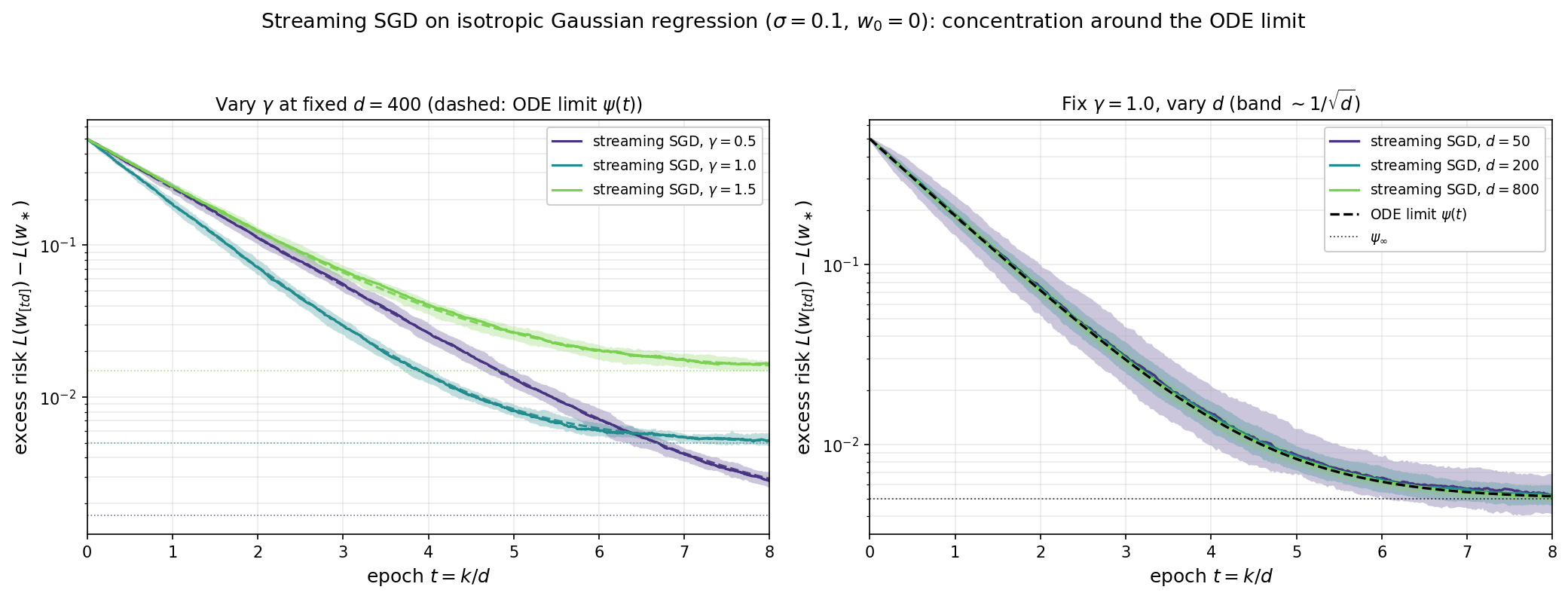
Concentration around the ODE limit
It remains to show that the loss itself $L(w_{[td]})$, rather than its expectation, concentrates around a deterministic limit. In order to establish this result, we require a few preliminaries on martingales and discrete approximation of ODE solutions. We begin with the following standard definition.
Definition (Square-integrable martingale). A sequence of random variables $(M_\ell)_{\ell\ge0}$ is a martingale if each $M_\ell$ is integrable ($\mathbb{E}\lvert M_\ell\rvert<\infty$) and its conditional expectation given the entire past equals its current value:
\[\mathbb{E}[M_{\ell+1}\mid M_0,M_1,\ldots,M_\ell]=M_\ell \qquad\text{for every }\ell\ge0.\]It is square-integrable if in addition $\mathbb{E}[M_\ell^2]<\infty$ for every $\ell\ge0$.
The next lemma bounds the supremum of a martingale by the second moment of its last term.
Lemma (Doob’s $L^2$ maximal inequality). Let $(M_\ell)_{\ell\ge0}$ be a square-integrable martingale with $M_0=0$. Then for every $n\ge0$, it holds:
\[\mathbb{E}\!\left[\max_{0\le \ell\le n} M_\ell^2\right] \;\le\; 4\,\mathbb{E}[M_n^2].\]Proof. Define $S_n:=\max_{0\le \ell\le n}\lvert M_\ell\rvert$. Our goal tail identity for the second moment:
\[\mathbb{E}[S_n^2]=\int_0^\infty 2\lambda\,\mathbb{P}(S_n\ge\lambda)\,d\lambda, \tag{47}\]which reduces the problem to controlling the tail $\mathbb{P}(S_n\ge\lambda)$ — the probability that the martingale reaches level $\lambda>0$ by time $n$. The crux of the proof is to show the maximal crossing estimate
\[\lambda\,\mathbb{P}(S_n\ge\lambda)\;\le\; \mathbb{E}\bigl[\lvert M_n\rvert\,\mathbf{1}_{\{S_n\ge\lambda\}}\bigr] \qquad\text{for every }\lambda>0. \tag{$\ast$}\]Proof of the crossing estimate $(\ast)$. We decompose the event ${S_n\ge\lambda}$ according to the first time the level $\lambda$ is reached. Namely, let $A_j$ be the event that the first crossing of level $\lambda$ occurs at time $j$:
\[A_j:=\{\lvert M_0\rvert<\lambda,\ldots,\lvert M_{j-1}\rvert<\lambda,\ \lvert M_j\rvert\ge\lambda\}.\]The events $A_0,\ldots,A_n$ are disjoint and their union is ${S_n\ge\lambda}$. On $A_j$ we have $\lvert M_j\rvert\ge\lambda$, and therefore
\[\lambda\,\mathbb{P}(A_j)\le \mathbb{E}\bigl[\lvert M_j\rvert\,\mathbf{1}_{A_j}\bigr].\]Because $A_j$ is determined by $M_0,\ldots,M_j$, iterating the martingale property gives $\mathbb{E}[M_n\mid M_0,\ldots,M_j]=M_j$ for every $n\ge j$. By Jensen’s inequality, we deduce
\[\lvert M_j\rvert=\bigl\lvert\mathbb{E}[M_n\mid M_0,\ldots,M_j]\bigr\rvert \le \mathbb{E}\bigl[\lvert M_n\rvert\mid M_0,\ldots,M_j\bigr].\]Multiplying by $\mathbf{1}_{A_j}$ and taking expectations yields
\[\mathbb{E}\bigl[\lvert M_j\rvert\,\mathbf{1}_{A_j}\bigr] \le \mathbb{E}\bigl[\lvert M_n\rvert\,\mathbf{1}_{A_j}\bigr].\]Summing over $j=0,\ldots,n$ and using disjointness gives $(\ast)$.
Conclusion. Substituting $(\ast)$ into the identity $(47)$ and applying Cauchy–Schwarz, yields
\[\begin{aligned} \mathbb{E}[S_n^2] &= \int_0^\infty 2\lambda\,\mathbb{P}(S_n\ge\lambda)\,d\lambda \\ &\le 2\int_0^\infty \mathbb{E}\bigl[\lvert M_n\rvert\,\mathbf{1}_{\{S_n\ge\lambda\}}\bigr]\,d\lambda \\ &=2\,\mathbb{E}\bigl[\lvert M_n\rvert\,S_n\bigr] \le 2\,\bigl(\mathbb{E}[M_n^2]\bigr)^{1/2}\bigl(\mathbb{E}[S_n^2]\bigr)^{1/2}, \end{aligned}\]where the middle equality uses the pointwise identity
\[\int_0^\infty \mathbf{1}_{\{S_n\ge\lambda\}}\,d\lambda = S_n.\]If $\mathbb{E}[S_n^2]=0$ there is nothing to prove. Otherwise, divide by $\bigl(\mathbb{E}[S_n^2]\bigr)^{1/2}$ to get $\mathbb{E}[S_n^2]\le 4\,\mathbb{E}[M_n^2]$. Since $S_n^2=\max_{0\le\ell\le n}M_\ell^2$, this is the desired inequality. $\square$
Next, we will need the following helper lemma on growth of sequences. It can be understood as a discrete version of the observation that an estimate of the form $\dot{\phi}(t)\leq \phi(t)$ forces $\phi$ to grow at most exponentially in time $t$.
Lemma (Discrete Gronwall inequality). Let $a_0,\ldots,a_n$ be nonnegative numbers. Suppose that for some constants $B,C\ge0$, we have
\[a_\ell \;\le\; B + C\sum_{k=0}^{\ell-1}a_k, \qquad \forall\ell=0,\ldots,n.\]Then the estimate holds:
\[\max_{0\le\ell\le n}a_\ell \;\le\; B\,e^{Cn}.\]Proof. Define $ b_\ell:=B+C\sum_{k=0}^{\ell-1}a_k.$ Then we have $a_\ell\le b_\ell$ by assumption, and $b_{\ell}$ satisfies the identity
\[b_{\ell+1}=b_\ell+C\,a_\ell\le (1+C)b_\ell.\]Since $b_0=B$, induction gives
\[b_\ell\le B(1+C)^\ell\le B e^{C\ell}.\]We conclude $a_\ell\le b_\ell\le B e^{C\ell}\le B e^{Cn}$ for every $\ell\le n$, as claimed. $\square$
The main use of the discrete Gronwall inequality is to establish consistency of discrete approximations of an ODE solution. This is the content of the following lemma.
Lemma (Stability of approximate ODE solutions). Consider a function $G:\mathbb{R}\to\mathbb{R}$ that is Lipschitz continuous with constant $L_G$. Fix a stepsize $h>0$ and a horizon $T>0$, and set $t_\ell=\ell h$ and $n=\lfloor T/h\rfloor$. Suppose $\phi$ solves the ODE
\[\phi(t)=z_0+\int_0^t G(\phi(s))\,ds,\qquad \forall t\in[0,T],\]Consider a discrete curve $(z_\ell)_{0\le\ell\le n}$ satisfying
\[z_\ell=z_0+h\sum_{k=0}^{\ell-1}G(z_k)+\xi_\ell.\]Write $\varepsilon:=\max_{0\le\ell\le n}\lvert\xi_\ell\rvert$ for the largest residual and set $M:=\sup_{t\in[0,T]}\lvert G(\phi(t))\rvert$. Then the estimate holds:
\[\max_{0\le\ell\le n}\lvert z_\ell-\phi(t_\ell)\rvert\;\le\;\Bigl(\varepsilon+\tfrac{1}{2}L_G M T\,h\Bigr)\,e^{L_G T}.\]Proof. Subtract the integral equation for $\phi$ from the discrete equation for $z_\ell$. Defining $e_\ell:=z_\ell-\phi(t_\ell)$ and noting the equality $\int_0^{t_\ell}G(\phi(s))\,ds=\sum_{k=0}^{\ell-1}\int_{t_k}^{t_{k+1}}G(\phi(s))\,ds$, we thus obtain
\[e_\ell =h\sum_{k=0}^{\ell-1}\bigl[G(z_k)-G(\phi(t_k))\bigr]+\xi_\ell-\sum_{k=0}^{\ell-1}\int_{t_k}^{t_{k+1}}\bigl[G(\phi(s))-G(\phi(t_k))\bigr]\,ds.\]We bound the three terms in order. For the first, $L_G$-Lipschitzness gives $\lvert G(z_k)-G(\phi(t_k))\rvert\le L_G\lvert e_k\rvert$. For the second term, by assumption we have $\lvert\xi_\ell\rvert\le\varepsilon$. For the last term, Lipschitz continuity of $G$ together with $M$-Lipschitz continuity of $\phi$ gives
\[\Bigl\lvert\int_{t_k}^{t_{k+1}}\bigl[G(\phi(s))-G(\phi(t_k))\bigr]\,ds\Bigr\rvert \le L_G\int_{t_k}^{t_{k+1}}M\,(s-t_k)\,ds=\tfrac{1}{2}L_G M\,h^2,\]Observe that the $\ell\le n\le T/h$ such terms sum to at most $\tfrac{1}{2}L_G M T\,h$. Summarizing, we have obtained the estimate
\[\lvert e_\ell\rvert\le L_G h\sum_{k=0}^{\ell-1}\lvert e_k\rvert+\varepsilon+\tfrac{1}{2}L_G M T\,h.\]Apply the discrete Gronwall lemma with $C=L_G h$ and $B=\varepsilon+\tfrac{1}{2}L_G M T\,h$. Taking into account $Cn=L_G h\,\lfloor T/h\rfloor\le L_G T$, this yields
\[\max_{0\le\ell\le n}\lvert e_\ell\rvert\le\Bigl(\varepsilon+\tfrac{1}{2}L_G M T\,h\Bigr)e^{L_G T},\]as claimed. $\square$
We are now done with the preliminaries and are ready to prove the main result of the section.
Theorem 10.2 (Deterministic limit of the loss). Fix $0<\gamma<2$, $\sigma > 0$, and consider streaming SGD $(43)$ on the isotropic Gaussian model of Lemma 10.1 from a deterministic initialization $w_0$ whose initial loss converges, $L(w_0)\to\psi_0$ as $d\to\infty$. Let $\psi : [0,\infty) \to \mathbb{R}$ be the solution of $(46)$ with initial condition $\psi(0) = \psi_0$, given explicitly by $(46a)$. Then for every $T > 0$, it holds:
\[\sup_{t \in [0,T]}\,\bigl\lvert L(w_{[td]}) - \psi(t)\bigr\rvert \;\xrightarrow[d\to\infty]{\mathbb{P}}\; 0.\]Proof. Define $L_k := L(w_k)$ and define
\[G(u) := -2\gamma\,(u - L_\ast) + \gamma^2\,u\]to be the velocity field of the limiting ODE $(46)$, so that $\psi$ solves $\dot\psi=G(\psi)$ with $\psi(0)=\psi_0$. Note that $G$ is affine, hence globally Lipschitz with constant $L_G := \lvert\gamma^2 - 2\gamma\rvert$. Recall that Lemma 10.1 reads
\[\mathbb{E}_k[L_{k+1}-L_k] \;=\; \frac{1}{d}\,G(L_k) \;+\; r_k, \qquad r_k := \frac{\rho_k}{d^2},\]where, by Lemma 10.1, the remainder $r_k\ge0$ is determined by the first $k$ samples and satisfies $r_k\le 2\gamma^2 L_k/d^2$.
Strategy. We will rewrite the loss curve $L_\ell$ (with $\ell=\lfloor td\rfloor$) as an approximate Euler discretization of this ODE — that is, in the precise form required by the ODE-stability lemma above — and then show the residual is uniformly small. So that the moments below stay controlled, we fix a level $R$ and run the argument up to the stopping time
\[\tau_R:=\inf\{k:L_k>R\}.\]Every estimate below is therefore read for $\ell\le Td\wedge\tau_R$; at the very end we choose $R$ large enough that the stopping is asymptotically irrelevant.
Doob decomposition. Split each increment of $L$ into its conditional mean and a martingale difference:
\[\begin{aligned} L_{k+1} - L_k &= \mathbb{E}_k[L_{k+1}-L_k] +\Bigl((L_{k+1}-L_k)-\mathbb{E}_k[L_{k+1}-L_k]\Bigr) \\ &= \frac{1}{d}\,G(L_k)+r_k+\Delta_{k+1}, \end{aligned}\]where we define
\[\Delta_{k+1}:=(L_{k+1}-L_k)-\mathbb{E}_k[L_{k+1}-L_k]=L_{k+1}-\mathbb{E}_k[L_{k+1}].\]The partial sums $M_\ell := \sum_{k=0}^{\ell-1}\Delta_{k+1}$ clearly form a martingale. Summing the increment identity from $k=0$ to $\ell-1$ and setting $t_\ell:=\ell/d$ therefore gives
\[\begin{aligned} L_\ell &=\psi_0+\frac{1}{d}\sum_{k=0}^{\ell-1}G(L_k)+\xi_\ell, \qquad \forall\ell\le Td\wedge\tau_R, \\ \xi_\ell &:=(L_0-\psi_0)+M_\ell+\sum_{k=0}^{\ell-1}r_k, \end{aligned}\]where we have written $L_0=\psi_0+(L_0-\psi_0)$ so that the discrete curve starts at the same value $\psi_0=\psi(0)$ as the ODE. This is exactly the approximate integral equation of the ODE-stability lemma, with discrete curve $z_\ell=L_\ell$, velocity field $G$, stepsize $h=1/d$, and residual $\xi_\ell$. The whole proof now reduces to showing that the residual is uniformly small,
\[\sup_{\ell\le Td\wedge\tau_R}\lvert\xi_\ell\rvert\xrightarrow[d\to\infty]{\mathbb{P}}0.\]The residual has three pieces — the initial gap $L_0-\psi_0$, the finite-$d$ drift correction $\sum_k r_k$, and the martingale $M_\ell$ — which we treat in turn. The initial gap is deterministic and vanishes by hypothesis, since $\lvert L_0-\psi_0\rvert=\lvert L(w_0)-\psi_0\rvert\to0$.
Drift correction. Before the stopping time $L_k\le R$, each remainder obeys $0\le r_k\le 2\gamma^2 R/d^2$. Therefore, we deduce:
\[\sup_{\ell\le Td\wedge\tau_R}\;\sum_{k=0}^{\ell-1}r_k \;\le\; Td\cdot\frac{2\gamma^2 R}{d^2} \;=\;\frac{2\gamma^2 R\,T}{d}.\]Martingale piece. To control $M_\ell$ we need a second-moment bound on the increments, namely the fluctuation estimate
\[\mathbb{E}_k\bigl[(L_{k+1}-L_k)^2\bigr] \;\le\; \frac{C_R}{d^2} \qquad \text{whenever } L_k \le R.\]To prove it, write $v_k=w_k-w_\ast$ and $g_{k+1}=(v_k^\top x_{k+1}-\eta_{k+1})x_{k+1}$, so that
\[L_{k+1}-L_k =-\frac{\gamma}{d}\,\langle v_k,g_{k+1}\rangle+\frac{\gamma^2}{2d^2}\,\|g_{k+1}\|^2.\]If $L_k\le R$, then $|v_k|^2=2(L_k-L_\ast)$ is bounded by a constant depending only on $R$ and $\sigma$. The first term in the loss increment is controlled by
\[\begin{aligned} \mathbb{E}_k\bigl[\langle v_k,g_{k+1}\rangle^2\bigr] &= \mathbb{E}\bigl[((v_k^\top x)^2-\eta\,v_k^\top x)^2\bigr] \\ &= 3\|v_k\|^4+\sigma^2\|v_k\|^2 \\ &\le C_R. \end{aligned}\]For the second term, use $g_{k+1}=(v_k^\top x-\eta)x$. Since $v_k^\top x-\eta$ is Gaussian with variance $|v_k|^2+\sigma^2\le C_R$, its eighth moment is bounded by a constant depending only on $R$ and $\sigma$, while $\mathbb{E}|x|^8=O(d^4)$. By Cauchy–Schwarz,
\[\begin{aligned} \mathbb{E}_k\|g_{k+1}\|^4 &= \mathbb{E}\bigl[(v_k^\top x-\eta)^4\|x\|^4\bigr] \\ &\le \Bigl(\mathbb{E}(v_k^\top x-\eta)^8\Bigr)^{1/2}\Bigl(\mathbb{E}\|x\|^8\Bigr)^{1/2} \\ &\le C_R d^2. \end{aligned}\]Combining the two terms proves the claim:
\[\begin{aligned} \mathbb{E}_k\bigl[(L_{k+1}-L_k)^2\bigr] &\le \frac{2\gamma^2}{d^2}\,\mathbb{E}_k\bigl[\langle v_k,g_{k+1}\rangle^2\bigr] +\frac{\gamma^4}{2d^4}\,\mathbb{E}_k\|g_{k+1}\|^4 \\ &\le \frac{C_R}{d^2}. \end{aligned}\]Since the conditional variance is at most the conditional second moment, the increments $\Delta_{k+1}$ inherit the same bound:
\[\mathbb{E}_k[\Delta_{k+1}^2] \;\le\; \mathbb{E}_k\bigl[(L_{k+1}-L_k)^2\bigr] \;\le\; \frac{C_R}{d^2}.\]The martingale differences are orthogonal, so $\mathbb{E}[M_\ell^2] = \sum_{k=0}^{\ell-1}\mathbb{E}[\Delta_{k+1}^2]\le C_R \ell/d^2$ before the stopping time. Applying Doob’s $L^2$ maximal inequality above with $\ell\leq Td\wedge\tau_R$ gives $\mathbb{E}[\sup_{\ell\le Td\wedge\tau_R} M_\ell^2] \le 4C_R T/d$, hence
\[\sup_{\ell\le Td\wedge\tau_R}\,\lvert M_\ell\rvert \;\xrightarrow{\mathbb{P}}\; 0.\]Together with the $O(1/d)$ drift bound above, this proves $\sup_{\ell\le Td\wedge\tau_R}\lvert\xi_\ell\rvert\xrightarrow{\mathbb{P}}0$.
Comparison with the ODE. The ODE-stability lemma above now applies to the approximate integral equation, with discrete curve $z_\ell=L_\ell$, solution $\psi$, stepsize $h=1/d$, and residual $\varepsilon=\sup_{\ell\le Td\wedge\tau_R}\lvert\xi_\ell\rvert$; the constant $M=\sup_{t\in[0,T]}\lvert G(\psi(t))\rvert$ is finite because $\psi$ is bounded on $[0,T]$ and $G$ is affine. The lemma bounds the discrepancy by $\bigl(\varepsilon+O(1/d)\bigr)e^{L_G T}$, and since $\varepsilon\xrightarrow{\mathbb{P}}0$ we conclude
\[\sup_{\ell\le Td\wedge\tau_R}\lvert L_\ell-\psi(t_\ell)\rvert \xrightarrow[d\to\infty]{\mathbb{P}}0.\]This proves concentration around $\psi$ up to the stopping level $R$. It remains to check that, for a large enough fixed $R$, the stopping time is unlikely to occur.
Because $0<\gamma<2$, the explicit formula $(46a)$ shows that $\psi$ is bounded on the time interval $[0,T]$:
\[B_T:=\sup_{0\le t\le T}\psi(t)<\infty.\]Choose $R>B_T+1$. If the stopped process exits before time $Td$, meaning $\tau_R\le Td$, then by definition $L_{\tau_R}>R$. On the other hand, $\psi(\tau_R/d)\le B_T$. Therefore, on the event ${\tau_R\le Td}$, we have
\[\sup_{\ell\le Td\wedge\tau_R}\lvert L_\ell-\psi(t_\ell)\rvert \ge \lvert L_{\tau_R}-\psi(\tau_R/d)\rvert > R-B_T > 1.\]On the other hand, the stopped convergence proved above says that the left-hand side converges to zero in probability. Hence $\mathbb{P}(\tau_R\le Td)\to0$. With probability tending to one, the stopped and unstopped processes agree on the whole interval $[0,T]$, so the unstopped convergence follows, completing the proof. $\square$
Failure of the scalar reduction for correlated features
Theorem 10.2 relies crucially on the fact that the conditional drift of $L(w_k)$ in the isotropic Gaussian model is itself a function of $L(w_k)$ (Lemma 10.1), which is what allowed us to compare the discrete chain to a scalar autonomous ODE. This property breaks for correlated features $x \sim \mathcal{N}(0, H)$ with $H \neq I_d$. Namely, a quick computation shows that the analogue of Lemma 10.1 takes the form
\[d\,\mathbb{E}_k\bigl[L(w_{k+1}) - L(w_k)\bigr] \;=\; -\gamma\,(w_k-w_\ast)^\top H^2 (w_k-w_\ast) \;+\; O(d^{-1}).\]The leading term involves the second spectral moment $(w-w_\ast)^\top H^2 (w-w_\ast)$, which is not a function of the excess loss $L - L_\ast = \tfrac{1}{2}(w-w_\ast)^\top H (w-w_\ast)$. Tracking the second spectral moment as an additional scalar does not help either: its drift involves the third moment $(w-w_\ast)^\top H^3 (w-w_\ast)$, and so on. Indeed, no finite collection of polynomial functions of $w_k$ allows one to rewrite the dynamics in a self-consistent (closed) way. Each new scalar statistic spawns another with a higher power of $H$, so any closed description must retain the entire spectrum of $H$. We will now try to side-step this issue by establishing the following
This motivates the two-step program for the rest of the section:
- Approximate SGD by an SDE. Keep the full $d$-dimensional iterate as the state and approximate it (in a rigorous sense) by a continuous-time process — homogenized SGD.
- Find the limiting risk curve. We will then see that the risk itself has a deterministic high-dimensional limit, described by a closed Volterra integro-differential equation which encodes the full spectrum of $H$ — precisely the information no finite set of scalar statistics can capture.
These two results are quite difficult to prove. Therefore, instead of providing formal proofs, we will focus on developing an informal intuition and motivation.
Throughout, we focus on the following Gaussian model of the data.
Assumption 10.3 (Gaussian streaming data). Each sample $(x,y)$ is drawn independently with
(i) Gaussian features $x \sim \mathcal N(0, H)$, where $H := \mathbb{E}[xx^\top]$ has operator norm bounded by a quantity that is independent of $d$;
(ii) labels are $y = \langle x, w_\ast\rangle + \zeta$ with $\zeta \sim \mathcal N(0,\sigma^2)$ independent of $x$;
(iii) bounded signal: $\lVert w_\ast\rVert$ is bounded by a quantity independent of $d$.
Forming a companion SDE by moment matching
It helps to first recall the general heuristic that links a discrete stochastic recursion to a continuous-time process. Suppose a discrete stochastic process evolves by small random increments $w_{k+1}=w_k+\Delta_k$. Suppose that the natural unit of time packs many steps together — here a single epoch $t=k/d$ contains $\sim d$ steps, each of size $O(1/d)$. Attach the time $\Delta t = 1/d$ to a single step, and split each increment into its conditional mean and a mean-zero fluctuation:
\[w_{k+1}=w_k+\underbrace{\mathbb{E}_k[\Delta_k]}_{=\;b(w_k)\,\Delta t}+\underbrace{\xi_k}_{\text{mean-zero}}, \qquad \operatorname{Cov}_k(\xi_k)=\Sigma(w_k)\,\Delta t.\]The first piece is a deterministic drift step whose direction $b(w_k)$ is a function of the current iterate $w_k$ and the second is a random fluctuation. This suggests approximating the process by the stochastic differential equation (SDE)
\[dX_t=b(X_t)\,dt+\Sigma(X_t)^{1/2}\,dB_t,\]whose drift and diffusion are exactly the per-step conditional mean and covariance measured per unit time:
For readers unfamiliar with SDEs, the differential $dX_t=b(X_t)\,dt+\Sigma(X_t)^{1/2}\,dB_t$ is shorthand for a precise statement about small increments, driven by Brownian motion $B_t$ — the continuous-path process with $B_0=0$ whose increments $B_t-B_s$ (for $s<t$) are independent of the past and Gaussian with mean zero and covariance $(t-s)I$. Concretely, the equation means that conditionally on $X_t$, the increment over a small time $h$ satisfies
\[\mathbb{E}\bigl[X_{t+h}-X_t\mid X_t\bigr]=b(X_t)\,h+o(h), \qquad \operatorname{Cov}\bigl[X_{t+h}-X_t\mid X_t\bigr]=\Sigma(X_t)\,h+o(h),\]and that the increment is Gaussian in the limit $h\to0$. A simple way to simulate the SDE is with the Euler–Maruyama step $X_{t+h}-X_t\approx b(X_t)\,h+\Sigma(X_t)^{1/2}(B_{t+h}-B_t)$. Reading the drift $b$ and diffusion $\Sigma$ off the one-step conditional mean and covariance of SGD — as in the display above, with $\Delta t$ in place of $h$ — is the recipe called moment matching (or the diffusion approximation).
The two ingredients are illustrated below. On the left is a pure planar Brownian motion $B_t$ — the driftless noise that drives the SDE. On the right is one trajectory of the moment-matched diffusion approximation $X_t$ of SGD on an anisotropic least-squares quadratic in $\mathbb{R}^2$: the path drifts toward the minimizer $w_\ast$ while fluctuating — drift plus Brownian noise, exactly the two terms of the SDE.
It cannot be overstressed that the correspondence arising from moment matching is purely heuristic. Matching the first two infinitesimal moments makes a particular SDE plausible as a limit, but it proves nothing on its own: the argument ignores the non-Gaussianity of individual steps, the higher-order moments, and — most importantly — how all of these errors accumulate over the $\sim d$ steps that make up one epoch. Whether the process and the SDE actually remain close, and in what sense and at what rate, is a separate question that must be settled by a theorem.
Diffusion approximation of SGD. Let us now implement the moment matching technique for the SGD iterates. To this end, write $u_k:=w_k-w_\ast$ for the centered iterate, and let the stochastic gradient and the one-step displacement be
\[g_{k+1}=(\langle w_k,x_{k+1}\rangle-y_{k+1})\,x_{k+1}, \qquad \Delta_k:=w_{k+1}-w_k=-\frac{\gamma}{d}\,g_{k+1}.\]Taking conditional expectations $\mathbb{E}_k$ over the fresh sample, a quick computation shows
\[\mathbb{E}_k[g_{k+1}]=Hu_k=\nabla L(w_k), \qquad \mathbb{E}_k\bigl[g_{k+1}g_{k+1}^\top\bigr]=\mathbb{E}\bigl[(x^\top u_k)^2\,xx^\top\bigr]+\sigma^2 H.\]Since $x$ is Gaussian, an elementary computation (Wick’s formula) gives the exact identity $\mathbb{E}[(x^\top u)^2xx^\top]=(u^\top Hu)\,H+2Hu u^\top H$. Combined with the expression $2L(w)=\sigma^2+u^\top Hu$ this yields
\[\mathbb{E}_k[\Delta_k]=-\frac{\gamma}{d}\,\nabla L(w_k), \qquad \mathbb{E}_k\bigl[\Delta_k\Delta_k^\top\bigr]=\frac{\gamma^2}{d^2}\Bigl(2L(w_k)\,H+2Hu_ku_k^\top H\Bigr).\]Moment matching now reads the drift and diffusion straight off the step. The drift is the conditional mean per unit time:
\[b(w_k)=d\,\mathbb{E}_k[\Delta_k]=-\gamma\,\nabla L(w_k).\]The diffusion is the covariance of $\Delta_k$ per unit time:
\[\Sigma(w_k)=d\,\operatorname{Cov}_k(\Delta_k)=d\Bigl(\mathbb{E}_k[\Delta_k\Delta_k^\top]-\mathbb{E}_k[\Delta_k]\,\mathbb{E}_k[\Delta_k]^\top\Bigr)=\frac{\gamma^2}{d}\bigl(2L(w_k)H+Hu_ku_k^\top H\bigr).\]Thus the diffusion SDE is given by
\[dX_t=-\gamma\,\nabla L(X_t)\,dt+\frac{\gamma}{\sqrt d}\Bigl(2L(X_t)\,H+\nabla L(X_t)\nabla L(X_t)^\top \Bigr)^{1/2}\,dB_t.\]The diffusion above splits into two parts: a bulk term $\tfrac{\gamma^2}{d}\,2L(X_t)H$ spread across all eigendirections of $H$, and a rank-one correction $\nabla L(X_t)\nabla L(X_t)^\top$ acting along the single direction $\nabla L(X_t)$. The SDE built from the drift together with the bulk term alone is homogenized SGD (defined precisely below); the rank-one correction is dropped.
Numerical illustration. As an illustration, we take a correlated-feature model — covariance $H=Q\Lambda Q^\top$, where $\Lambda=\operatorname{diag}(\lambda_i)$ has eigenvalues $\lambda_i=i/d$ and $Q$ is a Haar-random rotation (so $H$ is not diagonal and the features are correlated across all coordinates, not axis-aligned), label noise $\sigma=0.1$, a fixed signal $w_\ast$ of norm $|w_\ast|=1$, and start $w_0=0$ — and overlay two excess-risk curves. The solid curves (with $10$–$90\%$ band over independent trials) are streaming SGD, $t\mapsto L(w_{[td]})-L(w_\ast)$. The dashed curves are the diffusion approximation $L(X_t)-L(w_\ast)$, with $X_t$ solving the diffusion SDE above, simulated by Euler–Maruyama on the epoch clock with step $h=1/d$. Left: at fixed dimension $d=512$, the SDE reproduces the SGD curve across stepsizes $\gamma\in{0.5,1,1.5}$, matching both the decay rate and the stochastic noise floor. Right: at fixed $\gamma=1$, the two curves lock together more tightly as $d$ grows while the $10$–$90\%$ band narrows like $1/\sqrt d$.
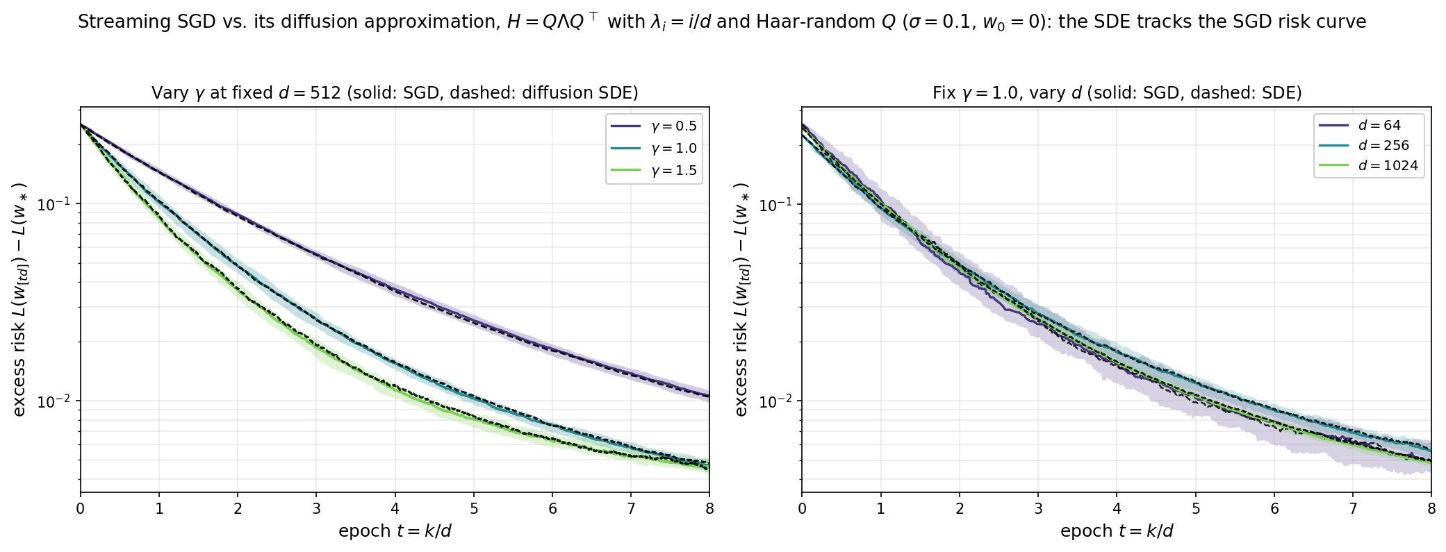
In what sense does the SDE approximate SGD?
We now have a candidate continuous-time process and numerical evidence that it tracks SGD. But in what precise sense does $X_t$ approximate $w_k$? Certainly in $\mathbb{R}^d$ the two processes are driven by different sources of randomness — so as vectors they never stay close; their difference $\lVert w_k-X_{k/d}\rVert$ stays of order one. The right notion is agreement of low-dimensional summaries. Instead of comparing the full vectors, we compare smooth scalar statistics evaluated along the two trajectories: for a test function $q:\mathbb{R}^d\to\mathbb{R}$ we ask whether
\[q(w_k)\;\approx\;q(X_{k/d}).\]These are exactly the observable quantities one cares about — the risk $L(w)=L(w_\ast)+\tfrac12(w-w_\ast)^\top H(w-w_\ast)$, squared norms, individual coordinates, projections onto fixed directions. We restrict to quadratic $q$: the natural and sufficient class, because it contains the risk, it is closed under the linear dynamics, and its second-order Taylor expansion is exact, leaving no higher-order remainder to control.
The plan for the rest of the section follows this idea. We first compute how a quadratic $q$ changes in one SGD step, and how it changes instantaneously along the candidate SDE — the latter through Itô’s formula. Comparing the two, the drift and the leading diffusion match exactly, and the only discrepancy is a single rank-one term of size $O(1/d)$, negligible in the limit. This pins down the process we keep — the definition of homogenized SGD — and culminates in the comparison result, Theorem 10.6, which makes “$q(w_k)\approx q(X_{k/d})$” quantitative.
Setting the stage, let $q\colon\mathbb{R}^d\to\mathbb{R}$ be any quadratic function. As usual, we identify one iteration step with a time increment $h=1/d$ on the epoch clock $t=k/d$. We compute the expected one-step change of $q$ along the discrete trajectory — its drift rate. Since $q$ is quadratic, its second-order Taylor expansion is exact:
\[\frac{1}{h}\,\mathbb{E}_k\bigl[q(w_{k+1})-q(w_k)\bigr] =d\,\nabla q(w_k)^\top\mathbb{E}_k[\Delta_k]+\frac{d}{2}\bigl\langle\nabla^2 q,\,\mathbb{E}_k[\Delta_k\Delta_k^\top]\bigr\rangle.\]Substituting the already computed expressions for the two moments of $\Delta_k$ yields
\[\frac{1}{h}\,\mathbb{E}_k\bigl[q(w_{k+1})-q(w_k)\bigr] =-\gamma\,\nabla q(w_k)^\top\nabla L(w_k) +\frac{\gamma^2 L(w_k)}{d}\operatorname{Tr}\!\bigl(H\nabla^2 q\bigr) +\frac{\gamma^2}{d}\,u_k^\top H\nabla^2 q\,Hu_k. \tag{48}\]The right-hand side of $(48)$ is the drift rate of the statistic $q$ under streaming SGD — how fast $\mathbb{E}_k\,q$ moves per unit of epoch time. The first two terms are of constant order: the gradient term $-\gamma\,\nabla q(w_k)^\top\nabla L(w_k)$ is $O(1)$, and although the second carries an explicit $1/d$, its trace $\operatorname{Tr}(H\nabla^2 q)$ sums contributions from all $\sim d$ eigendirections, so it too is $O(1)$. The third term is smaller: $u_k^\top H\nabla^2 q\,Hu_k$ is a single quadratic form, bounded once $|u_k|$ and $|H|$ are, so with the $1/d$ prefactor it is only $O(1/d)$. Thus the third term becomes negligible in high dimensions.
The plan now is to compute the analogous drift rate for the diffusion approximation. This is immediate from Ito’s calculus rule, summarized in the following lemma.
Lemma (Itô’s formula). Let $(X_t)_{t\ge0}$ solve the SDE $dX_t=b(X_t)\,dt+\Sigma(X_t)^{1/2}\,dB_t$ in $\mathbb{R}^d$, and let $q:\mathbb{R}^d\to\mathbb{R}$ be twice continuously differentiable. Then
\[dq(X_t)=\Bigl(\langle\nabla q(X_t),b(X_t)\rangle+\tfrac12\bigl\langle\nabla^2 q(X_t),\Sigma(X_t)\bigr\rangle\Bigr)\,dt+\nabla q(X_t)^\top\Sigma(X_t)^{1/2}\,dB_t.\]In particular the $dB_t$ term has conditional mean zero, so the deterministic drift of $q(X_t)$ is governed by the drift operator
\[\frac{d}{dt}\,\mathbb{E}\,q(X_t)=\mathbb{E}[\langle\nabla q(X_t),b(X_t)\rangle+\tfrac12\langle\nabla^2 q(X_t),\Sigma(X_t)\rangle].\]Applying the lemma to the diffusion SDE yields
\[\frac{d}{dt}\,\mathbb{E}\,q(X_t) =\mathbb{E}\Bigl[-\gamma\,\nabla q(X_t)^\top\nabla L(X_t) +\frac{\gamma^2 L(X_t)}{d}\operatorname{Tr}\!\bigl(H\nabla^2 q\bigr) +\frac{\gamma^2}{2d}\,u_t^\top H\nabla^2 q\,Hu_t\Bigr]. \tag{49}\]Inside the bracket of $(49)$, the first two terms are exactly the leading $O(1)$ part of the discrete drift rate $(48)$; the last — from the rank-one part of $\Sigma$ — is a single quadratic form of order $1/d$. So along the diffusion the expected statistic evolves at the same rate as along SGD, up to an $O(1/d)$ rank-one correction.
Since the rank-one term is $O(1/d)$, it has no effect on the leading-order evolution of any quadratic statistic both along SGD and the diffusion approximation. We may therefore discard it and keep only the bulk $\tfrac{\gamma^2}{d}\,2L(X)H$ in the covariance of the SDE. The resulting process is called the homogenized SGD and it is indistinguishable from the diffusion approximation in high dimensions on the level of quadratic statistics.
Definition 10.4 (Homogenized SGD). Homogenized SGD with stepsize $\gamma$ and feature covariance $H$ is the $\mathbb{R}^d$-valued continuous-time process $(X_t)_{t\ge 0}$ with $X_0 = w_0$ solving
\[dX_t = -\gamma\,\nabla L(X_t)\,dt + \gamma\,\sqrt{\tfrac{2\,L(X_t)\,H}{d}}\;dB_t. \tag{50}\]We can now state the central theorem showing that the evolution of quadratic statistics along SGD and the homogenized SGD are indistinguishable in high dimensions.
Theorem 10.6 (Streaming SGD vs. homogenized SGD). Under Assumption 10.3, for every quadratic $q : \mathbb{R}^d \to \mathbb{R}$, every $\varepsilon > 0$, and every deterministic initialization $w_0$ with $\lVert w_0\rVert \le 1$, there is a constant $C = C(\lVert H\rVert _{\mathrm{op}}, \varepsilon)$ such that for every $n \le d\log d/C$, the SGD iterates $\lbrace w_k\rbrace _{k=0}^n$ and the homogenized SGD process $\lbrace X_t\rbrace _{t=0}^{n/d}$ with the same initialization satisfy
\[\sup_{0\le k\le n}\bigl\lvert q(w_k) - q(X_{k/d})\bigr\rvert \;<\; \bigl(\|\nabla^2 q\|_{\mathrm{op}} + \|\nabla q(0)\|\bigr)\cdot e^{Cn/d}\cdot d^{-1/2 + \varepsilon}, \tag{51}\]with overwhelming probability.
Thus every quadratic statistic of streaming SGD agrees with its homogenized counterpart up to an order $O(d^{-1/2 + \varepsilon})$ error, uniformly over exponentially many steps.
The Volterra risk curve
We would like to now use the ODE in order to describe the entire risk curve $t\mapsto L(X_t)$ where $X_t$ is the homogenized SGD. The first step is to apply Ito’s formula with $q=L$ to deduce the expression:
\[dL(X_t) = \Bigl(\tfrac{\gamma^2}{d}\operatorname{Tr}(H^2)\,L(X_t) - \gamma\,u_t^\top H^2 u_t\Bigr)\,dt + \gamma\sqrt{\tfrac{2L(X_t)}{d}}\;u_t^\top H^{3/2}\,dB_t.\]where we set $u_t := X_t - w_\ast$. Taking expectations annihilates the martingale and leaves an evolution equation for the expected loss,
\[\frac{d}{dt}\,\mathbb{E}\,L(X_t) = \frac{\gamma^2}{d}\operatorname{Tr}(H^2)\,\mathbb{E}\,L(X_t) - \gamma\,\mathbb{E}\bigl[u_t^\top H^2 u_t\bigr].\]The problem is that this equation is not closed: the right-hand side involves $\mathbb{E}[u_t^\top H^2 u_t]$, which is not a function of $\mathbb{E}\,L(X_t)$ alone. A simple fix is that rather than monitoring the risk alone, we monitor all quadratic statistics simultaneously. Note that any quadratic form of $u_t$ can be written as a trace product ${\rm tr}(Au_tu_t^{\top})$ with respect to some symmetric matrix $A$, so its expectation is $\operatorname{tr}(A M_t)$ with $M_t := \mathbb{E}[u_tu_t^{\top}]$. It therefore suffices to track the evolution of the second-moment matrix $M_t$. In particular, the expected loss is recovered trivially by the formula
\[\mathbb{E}\,L(X_t) = \tfrac12\sigma^2 + \tfrac12\,\mathbb{E}\bigl[u_t^\top H u_t\bigr] = \tfrac12\sigma^2 + \tfrac12\operatorname{Tr}\!\bigl(H M_t\bigr).\]Applying Ito’s formula entrywise to $M_t$ yields the closed linear ODE for $M_t$:
\[\dot M_t = \underbrace{-\gamma\,(H M_t + M_t H)}_{\text{drift}} + \underbrace{\frac{2\gamma^2\,\mathbb{E}\,L(X_t)}{d}\,H}_{\text{diffusion } \Sigma}.\]This is a linear matrix ODE — a differential Lyapunov equation — and it can be solved by standard techniques: vectorize using $\operatorname{vec}(HM)=(I\otimes H)\operatorname{vec}M$ and $\operatorname{vec}(MH)=(H\otimes I)\operatorname{vec}M$ to obtain an ordinary linear system, then apply the variation of parameters method (see [Rug96, BBH19]). The end result is the following formula which describes $M_t$ in terms of an integral involving $M_s$ for $s<t$:
\[M_t = e^{-\gamma H t}\,M_0\,e^{-\gamma H t} + \int_0^t \frac{2\gamma^2\,\mathbb{E}\,L(X_s)}{d}\;e^{-\gamma H(t-s)}\,H\,e^{-\gamma H(t-s)}\,ds.\]Passing now to the expected loss yields a very simple evolution equation. Namely define
\[F(s) := \tfrac12\sigma^2 + \tfrac12(w_0-w_\ast)^\top H e^{-2 s H}(w_0-w_\ast), \tag{52}\]which is exactly the loss along the noiseless gradient flow $\dot Y_t = -\gamma\nabla L(Y_t)$. The loss along the homogenized SGD then evolves according to the expression
\[\mathbb{E}\,L(X_t) = F(\gamma t) + \int_0^t \frac{\gamma^2}{d}\operatorname{Tr}\!\bigl(H^2 e^{-2\gamma H(t-s)}\bigr)\,\mathbb{E}\,L(X_s)\,ds.\]This expression is an instance of a so-called Volterra renewal equation.
Definition 10.7 (Volterra risk model). With $F$ given by $(52)$ and the memory kernel
\[\mathcal{K}_\gamma(t) := \frac{\gamma^2}{d}\operatorname{Tr}\bigl(H^2\,e^{-2\gamma H t}\bigr), \tag{53}\]the Volterra risk model $\Psi : [0,\infty) \to [0,\infty)$ is the unique solution of
\[\Psi(t) = F(\gamma t) + \int_0^t \mathcal{K}_\gamma(t-s)\,\Psi(s)\,ds. \tag{54}\]Summarizing we have shown that the expected loss $\mathbb{E}L(w_k)$ along SGD is close to the expected loss $\mathbb{E}L(X_{k/d})$, with the latter being described by a solution of the Volterra integral equation $(54)$. Remarkably, the expectation can be dropped, yielding a deterministic equation for the loss that is an accurate approximation of the loss along the SGD iterates.
Theorem 10.8 (Volterra risk curve). Under Assumption 10.3, for every $T > 0$ and every $\varepsilon’ > 0$, the following holds:
\[\sup_{0\le t \le T}\bigl\lvert L(X_t) - \Psi(t)\bigr\rvert \;<\; C(T, \|H\|_{\mathrm{op}})\cdot d^{-1/2 + \varepsilon'}, \tag{55}\]with overwhelming probability.
Combining Theorems 10.6 and 10.8 gives the end-to-end statement: on the epoch scale $t = k/d$, and up to errors of order $d^{-1/2 + O(\varepsilon)}$, the random risk curve $L(w_{[td]})$ of streaming SGD agrees with the deterministic Volterra solution $\Psi(t)$.
It is worth making explicit what the limiting curve actually depends on, because the high-dimensional problem enters $(54)$ only through the spectrum of $H$. Write the eigendecomposition $H = \sum_{i=1}^d \lambda_i\, v_i v_i^\top$, with eigenvalues $\lambda_1,\ldots,\lambda_d \ge 0$ and orthonormal eigenvectors $v_i$, and collect the eigenvalues in the empirical spectral measure
\[\mu_H := \frac1d\sum_{i=1}^d \delta_{\lambda_i}.\]The memory kernel is then exactly a Laplace-type transform of $\mu_H$:
\[\mathcal{K}_\gamma(t) = \frac{\gamma^2}{d}\operatorname{Tr}\!\bigl(H^2 e^{-2\gamma H t}\bigr) = \gamma^2 \int_0^\infty \lambda^2 e^{-2\gamma\lambda t}\,\mu_H(d\lambda). \tag{56}\]The forcing carries the same spectral structure, now weighted by how the initialization error $u_0 := w_0 - w_\ast$ aligns with the eigendirections. Setting $c_i := \langle v_i, u_0\rangle$ and defining the signal-weighted spectral measure $\nu := \sum_{i=1}^d c_i^2\,\delta_{\lambda_i}$ (of total mass $\nu(\mathbb{R}) = |u_0|^2$), the gradient-flow risk $(52)$ becomes
\[F(s) = \tfrac12\sigma^2 + \tfrac12\int_0^\infty \lambda\, e^{-2 s\lambda}\,\nu(d\lambda). \tag{57}\]Hence the entire limiting risk curve — kernel, forcing, and therefore the solution $\Psi$ of $(54)$ — is a deterministic functional of the two spectral statistics $(\mu_H, \nu)$; the ambient dimension $d$ enters nowhere else. In particular, if these measures converge as $d\to\infty$ — for instance $\mu_H$ to the Marchenko–Pastur law of Section 7, with the signal spread isotropically so that $\nu$ converges as well — then $\mathcal{K}_\gamma$, $F$, and $\Psi$ converge, and the limiting risk curve is dimension-free.
This closes the loop with the deterministic theory of Section 7. There, the average-case complexity of gradient descent and conjugate gradients on a quadratic was dictated by the spectral density of the Hessian, with the small-eigenvalue (soft-edge) behavior fixing the asymptotic rate. The same spectral data now governs the high-dimensional limit of streaming SGD: the forcing $F$ is the noiseless gradient-flow risk — the continuous-time, full-gradient object of Section 7, read off the very same integrals $(57)$ — while the convolution in $(54)$ layers on the accumulated effect of the one-pass gradient noise, again as a spectral integral $(56)$ against $\mu_H$.
Numerical illustration. The figure below uses the same correlated-feature model as above — covariance $H = Q\Lambda Q^\top$ with $\Lambda = \operatorname{diag}(\lambda_i)$, $\lambda_i = i/d$ (linear-ramp spectrum on $(0,1]$) and $Q$ a Haar-random rotation, label noise $\sigma = 0.1$, a unit signal $|w_\ast| = 1$, and start $w_0 = 0$. In both panels the colored curve is the median of $t\mapsto L(w_{[td]}) - L(w_\ast)$ over independent trials, the shaded ribbon is the corresponding $10$–$90\%$ interquantile band, and the black curve is the deterministic Volterra solution $\Psi(t) - \tfrac12\sigma^2$ obtained by trapezoidal-rule integration of $(54)$ with the limiting spectral data of $(56)$–$(57)$ (evaluated at $d = 1024$ as a proxy for the limit). Left: at fixed dimension $d = 512$, the Volterra curve tracks streaming SGD across stepsizes $\gamma \in \lbrace 0.5, 1, 1.5\rbrace$, capturing both the decay rate and the noise floor. Right: at fixed $\gamma = 1$, as $d \in \lbrace 50, 200, 800, 3200\rbrace$ grows the bands shrink around the single deterministic Volterra curve, exactly as Theorem 10.8 predicts.
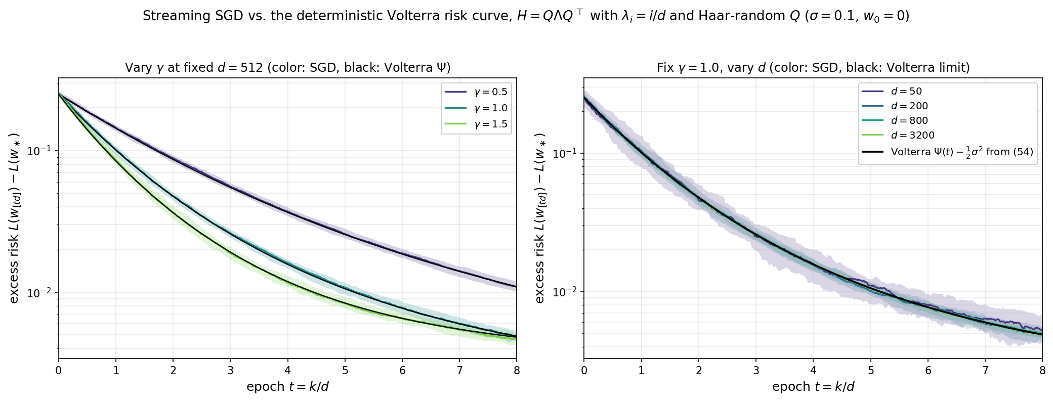
Reading off consequences. There are now a number of observations we cn extract from the Volterra equation $(54)$ that apply to the streaming SGD. Throughout, write $\bar\lambda := \int \lambda\,\mu_H(d\lambda) = \tfrac{1}{d}\operatorname{Tr} H$ for the average eigenvalue of $H$.
1. Critical stepsize. Let us first compute the maximal stepsize $\gamma$ that keeps the Volterra model bounded. To this end, a direct computation shows that the total mass of the memory kernel is
\[\int_0^\infty \mathcal{K}_\gamma(t)\,dt \;=\; \gamma^2 \int \int_0^\infty \lambda^2\, e^{-2\gamma\lambda t}\,dt\,\mu_H(d\lambda) \;=\; \gamma^2 \int \frac{\lambda^2}{2\gamma\lambda}\,\mu_H(d\lambda) \;=\; \frac{\gamma\bar\lambda}{2}. \tag{58}\]Define now the convolution operation $(f * g)(t) := \int_0^t f(t-s)\,g(s)\,ds$, so that $(54)$ reads as $\Psi = F(\gamma\,\cdot) + \mathcal{K}_\gamma * \Psi$. Substituting the equation into itself $n$ times unrolls it into
\[\Psi \;=\; F(\gamma\,\cdot) \;+\; \mathcal{K}_\gamma * F(\gamma\,\cdot) \;+\; \mathcal{K}_\gamma^{*2} * F(\gamma\,\cdot) \;+\; \cdots \;+\; \mathcal{K}_\gamma^{*n} * F(\gamma\,\cdot) \;+\; \mathcal{K}_\gamma^{*(n+1)} * \Psi,\]where $\mathcal{K}_\gamma^{*n} := \mathcal{K}_\gamma * \cdots * \mathcal{K}_\gamma$ is the $n$-fold convolution. Each term in this sum is controlled by the kernel mass. Indeed, since we have $\mathcal{K}_\gamma \ge 0$ and $F \le F(0)$, we obtain
\[\sup_{t \ge 0}\;\bigl(\mathcal{K}_\gamma^{*n} * F(\gamma\,\cdot)\bigr)(t) \;\le\; F(0)\int_0^\infty \mathcal{K}_\gamma^{*n}(t)\,dt \;=\; F(0)\Bigl(\frac{\gamma\bar\lambda}{2}\Bigr)^{\!n},\]where the last equality uses that the integral of a convolution is the product of the integrals. If the mass $\gamma\bar\lambda/2$ is $< 1$, these bounds form a convergent geometric series and the remainder term vanishes as $n \to \infty$, leaving the Neumann series $\Psi = \sum_{n\ge0} \mathcal{K}_\gamma^{*n} * F(\gamma\,\cdot)$ with $\sup_t \Psi(t) \le F(0)/(1 - \gamma\bar\lambda/2)$. If instead the mass is $\ge 1$ each term satisfies $(\mathcal{K}_\gamma^{*n} * F(\gamma\,\cdot))(t) \ge \tfrac12\sigma^2 \int_0^t \mathcal{K}_\gamma^{*n}(s)\,ds \to \tfrac12\sigma^2\,(\gamma\bar\lambda/2)^n$ as $t \to \infty$, so infinitely many terms each contribute at least $\tfrac12\sigma^2$, and $\Psi(t) \to \infty$. Streaming SGD therefore has a critical stepsize:
\[\Psi \text{ remains bounded} \quad\Longleftrightarrow\quad \gamma \;<\; \gamma_c := \frac{2}{\bar\lambda} = \frac{2d}{\operatorname{Tr} H}.\]Thus, stability is governed by the average eigenvalue — the aggregate gradient noise generated across the whole spectrum — and not by $\lambda_{\max}$. Indeed, with stepsize $\gamma/d$, the classical curvature constraint of gradient descent reads $\gamma < 2d/\lambda_{\max}$. For the isotropic model $H = I$ we recover the threshold $\gamma_c = 2$ of the scalar ODE $(46)$.
2. The noise floor. Consider the stable regime $\gamma < \gamma_c$, so that $\Psi$ is bounded. Let us compute the value $\Psi(\infty) := \lim_{t\to\infty}\Psi(t)$ that the risk settles at (taking for granted that the limit exists, which can be justified). We pass to the limit $t \to \infty$ on both sides of $(54)$. From the expression $(57)$ we have $F(\gamma t) = \tfrac12\sigma^2 + \tfrac12\int \lambda\, e^{-2\gamma t\lambda}\,\nu(d\lambda)$, and therefore $F(\gamma t) \to \tfrac12\sigma^2$.
Next consider the convolution term. We change variables $u := t - s$ to put the kernel’s argument in the integrand:
\[\int_0^t \mathcal{K}_\gamma(t-s)\,\Psi(s)\,ds \;=\; \int_0^t \mathcal{K}_\gamma(u)\,\Psi(t-u)\,du.\]As $t \to \infty$, the factor $\Psi(t-u)$ tends to $\Psi(\infty)$ for every fixed $u$; since $\Psi$ is bounded and $\mathcal{K}_\gamma$ is integrable, dominated convergence lets us pass the limit inside, and the right-hand side converges to $\Psi(\infty)\int_0^\infty \mathcal{K}_\gamma(u)\,du = \Psi(\infty)\cdot\tfrac{\gamma\bar\lambda}{2}$ by $(58)$.
Thus in the limit $t\to \infty$ the Volterra equation collapses to a scalar fixed-point equation:
\[\Psi(\infty) \;=\; \tfrac12\sigma^2 + \frac{\gamma\bar\lambda}{2}\,\Psi(\infty) \qquad\Longrightarrow\qquad \Psi(\infty) - \tfrac12\sigma^2 \;=\; \frac{\gamma\bar\lambda\,\sigma^2}{2\,(2 - \gamma\bar\lambda)}. \tag{59}\]The floor is proportional to $\gamma$ for small stepsizes and blows up as $\gamma \uparrow \gamma_c$. For $H = I$ it reduces to $\gamma\sigma^2/(2(2-\gamma))$, matching exactly the stationary value of the scalar ODE $(46)$.
3. Rate of convergence and stepsize criticality. At what exponential rate does $\Psi(t)$ approach its floor? Suppose as an ansatz that for large $t$ we have $\Psi(t) = \Psi(\infty) + C e^{-\lambda^* t}$ for some value $\lambda^* > 0$ and a constant $C \ne 0$, and substitute this guess into $(54)$. With the change of variables $u := t - s$, as in item 2, the convolution term splits into a constant piece and an exponential piece:
\[\int_0^t \mathcal{K}_\gamma(t-s)\,\Psi(s)\,ds \;=\; \Psi(\infty)\int_0^t \mathcal{K}_\gamma(u)\,du \;+\; C\,e^{-\lambda^* t}\int_0^t e^{\lambda^* u}\,\mathcal{K}_\gamma(u)\,du.\]Now let $t$ grow and compare the two sides of $(54)$ order by order. The constant terms reproduce the fixed-point equation of item 2 and cancel. Assuming the forcing decays faster than the ansatz (more on this below), the surviving terms of order $e^{-\lambda^* t}$ read
\[C\,e^{-\lambda^* t} \;=\; C\,e^{-\lambda^* t}\int_0^\infty e^{\lambda^* u}\,\mathcal{K}_\gamma(u)\,du.\]Dividing through by $C e^{-\lambda^* t}$ forces the consistency condition
\[\int_0^\infty e^{\lambda^* t}\,\mathcal{K}_\gamma(t)\,dt \;=\; \gamma^2 \int\int_0^\infty \lambda^2\, e^{-(2\gamma\lambda - \lambda^*)t}\,dt\,\mu_H(d\lambda) \;=\; \gamma^2 \int \frac{\lambda^2}{2\gamma\lambda - \lambda^*}\,\mu_H(d\lambda) \;=\; 1, \tag{60}\]where the $t$-integral is computed as in $(58)$ and converges precisely when $\lambda^* < 2\gamma\lambda_{\min}$, with $\lambda_{\min} := \min_i \lambda_i(H)$. This restriction is exactly the standing assumption above: the forcing decays at the gradient-flow rate, $F(\gamma t) - \tfrac12\sigma^2 \sim e^{-2\gamma\lambda_{\min}t}$ by $(57)$, so it is negligible at order $e^{-\lambda^* t}$ only when $\lambda^* < 2\gamma\lambda_{\min}$. The root $\lambda^*(\gamma) \in (0, 2\gamma\lambda_{\min})$ of $(60)$ is the decay rate of the risk when it exists; when no root exists the noise is subdominant and the rate is that of the forcing $2\gamma\lambda_{\min}$.
4. Critical batch size (informal). Mini-batching (Section 8) averages $B$ independent gradients per update, leaving the drift unchanged and dividing the memory kernel by $B$. Therefore the critical stepsize becomes
\[\gamma_c(B) \;=\; \frac{2B}{\bar\lambda}.\]However, we also know that due to discretization effects in the noiseless setting, we can not allow a stepsize larger than $\gamma= 2d/\lambda_{\max}(H)$. Equating the two quantities yields the critical batch size
\[B_{\mathrm{crit}} \;=\; \frac{d\,\bar\lambda}{\lambda_{\max}} \;=\; \frac{\operatorname{Tr} H}{\lambda_{\max}(H)},\]One expects that past this threshold, larger batch sizes have a limited effect. This intuition can be made formal by showing that precisely at the value $B_{\mathrm{crit}}$, the discrete dynamics transition from noise-dominated to problem-dominated regimes. The complete argument based on a discrete Volterra equation can be found in [Lee+22].
Numerical illustration. The figure below exhibits this transition on the correlated-feature model of this section ($H = Q\Lambda Q^\top$, $\lambda_i = i/d$, Haar-random $Q$, $d = 1024$, $\sigma = 0.1$, $|w_\ast| = 1$, $w_0 = 0$), for which $\bar\lambda \approx \tfrac12$, $\lambda_{\max} = 1$, and hence $B_{\mathrm{crit}} = \operatorname{Tr}H/\lambda_{\max} \approx d/2 = 512$. For each batch size $B$, mini-batch streaming SGD is run at the stepsize $\gamma(B) = \tfrac18\min\lbrace 2B/\bar\lambda,\ 2d/\lambda_{\max}\rbrace$, and we record the number of updates needed to reach the excess risk $\varepsilon = 3\times 10^{-3}$. Below $B_{\mathrm{crit}}$ the count falls like $1/B$ (linear speedup, dashed guide); at $B_{\mathrm{crit}}$ (vertical line) it bends and plateaus, matching the update count of full-batch gradient descent run at the curvature-limited stepsize (dotted line). Larger batches past this point leave the iteration count unchanged.
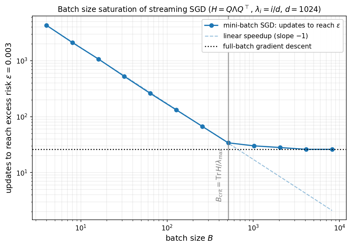
The scalar-ODE reduction of Theorem 10.2 is in the spirit of Ben Arous, Gheissari, and Jagannath [BAGJ22] and goes back, in the neural-network context, to Saad and Solla [SS95]. The homogenized SGD comparison and the Volterra risk curve are due to Paquette, Paquette, Adlam, and Pennington [Paq+22a, Paq+22b], with extensions in Collins-Woodfin and Paquette [CP23]. The stepsize-criticality analysis of the Volterra equation appears in Paquette, Lee, Pedregosa, and Paquette [PLPP21], and the batch-size saturation analysis in Lee, Cheng, Paquette, and Paquette [Lee+22]. We have followed the lecture-note synthesis of Paquette [Paq23].
11. Related Literature
The results discussed in these notes are largely classical in numerical optimization, Krylov methods, inverse problems, and random matrix theory. The novelty of these notes is mostly synthesis and alignment of viewpoints: optimization complexity bounds, Krylov polynomial optimality, source-condition regularity, and random-matrix spectral asymptotics are presented in one unified quadratic framework.
- Gradient descent and first-order complexity. Linear-rate GD analysis for strongly convex quadratics and condition-number dependence are standard; see [Pol64, Nes04, Nes18].
- Chebyshev acceleration and semi-iterative methods. The minimax polynomial viewpoint and Chebyshev stepsizes are classical; see [Var62, You71, Saa03].
- Conjugate gradient and Krylov optimality. Foundational CG/Krylov results originate in [HS52, Lan52]; modern treatments include [Saa03, Gre97].
- Source conditions and spectral-decay rates. The source-condition framework and decay-dependent rates are standard in inverse problems and regularization theory; see [EHN96, Han95].
- Marchenko–Pastur asymptotics. The limiting spectral law is due to [MP67], with modern expositions in [BS10, Ver18].
- Average-case optimization complexity. The spectral-integral viewpoint used throughout Section 7 is closely tied to the average-case analysis framework developed by Pedregosa, Scieur, and Paquette and collaborators [PS20, SP20, PvMPP21, CGPSP22]: convergence rates are governed by the limiting spectral density of the Hessian rather than by extremal eigenvalues alone, and the edge/tail behavior of this density determines the asymptotic exponent.
- Stochastic gradient descent for least squares. The constant-stepsize, tail-averaged SGD analysis in Section 8 follows the Markov-chain/covariance approach of [JKK+18], which establishes minimax optimality of tail-averaged SGD for the linear regression problem.
- Lower bounds for first-order methods. The tridiagonal chain quadratic and the rotation argument behind Lemma 9.1 and Theorem 9.2 are due to Nemirovski and Yudin [NY83]; modern textbook treatments appear in Nesterov [Nes04, Nes18]. The same construction yields the matching $\Omega(\sqrt{\kappa}\,\log(1/\varepsilon))$ lower bound for general smooth strongly convex minimization beyond the quadratic class.
- Lower bounds for stochastic algorithms on least squares. The matching minimax lower bound in Theorem 9.9 is the well-specified Gaussian-noise instance of the classical $\sigma^2 d/n$ minimax bound for fixed-design linear regression; we follow the elegant Bayesian-Gaussian-prior proof of Mourtada [Mou22].
- Interpolation and randomized Kaczmarz. The randomized Kaczmarz algorithm of Theorem 8.5 is due to Strohmer and Vershynin [SV09], building on the classical cyclic method of Kaczmarz [Kac37]; the connection between Kaczmarz and importance-sampled SGD on interpolation least squares was articulated by Needell, Srebro, and Ward [NSW16], and the broader family of randomized iterative methods is unified by Gower and Richtárik [GR15].
- High-dimensional limits of streaming SGD. The scalar-ODE reduction in §10.1–10.2 is an old idea in the physics literature on two-layer neural networks going back to Saad and Solla [SS95], and has been given a rigorous and general formulation by Ben Arous, Gheissari, and Jagannath [BAGJ22]. The homogenized-SGD SDE and the Volterra risk curve of §10.3–10.5 are due to Paquette, Paquette, Adlam, and Pennington [Paq+22a] and were further developed in [Paq+22b, CP23]; the lecture notes [Paq23] provide the expository synthesis we have followed.
References
- [HS52] Hestenes, M. R., and Stiefel, E. (1952). Methods of conjugate gradients for solving linear systems. Journal of Research of the National Bureau of Standards.
- [Lan52] Lanczos, C. (1952). An iteration method for the solution of the eigenvalue problem of linear differential and integral operators. Journal of Research of the National Bureau of Standards.
- [Pol64] Polyak, B. T. (1964). Some methods of speeding up the convergence of iteration methods. USSR Computational Mathematics and Mathematical Physics.
- [Var62] Varga, R. S. (1962). Matrix Iterative Analysis. Prentice-Hall.
- [You71] Young, D. M. (1971). Iterative Solution of Large Linear Systems. Academic Press.
- [EHN96] Engl, H. W., Hanke, M., and Neubauer, A. (1996). Regularization of Inverse Problems. Kluwer.
- [Han95] Hanke, M. (1995). Conjugate Gradient Type Methods for Ill-Posed Problems. Longman.
- [Saa03] Saad, Y. (2003). Iterative Methods for Sparse Linear Systems (2nd ed.). SIAM.
- [Gre97] Greenbaum, A. (1997). Iterative Methods for Solving Linear Systems. SIAM.
- [MP67] Marchenko, V. A., and Pastur, L. A. (1967). Distribution of eigenvalues for some sets of random matrices. Mathematics of the USSR-Sbornik.
- [BS10] Bai, Z. D., and Silverstein, J. W. (2010). Spectral Analysis of Large Dimensional Random Matrices (2nd ed.). Springer.
- [Nes04] Nesterov, Y. (2004). Introductory Lectures on Convex Optimization. Kluwer.
- [Nes18] Nesterov, Y. (2018). Lectures on Convex Optimization (2nd ed.). Springer.
- [NY83] Nemirovski, A. S., and Yudin, D. B. (1983). Problem Complexity and Method Efficiency in Optimization. Wiley-Interscience.
- [Ver18] Vershynin, R. (2018). High-Dimensional Probability. Cambridge University Press.
- [PS20] Pedregosa, F., and Scieur, D. (2020). Acceleration through spectral density estimation. Proceedings of the 37th International Conference on Machine Learning, PMLR 119:7553–7562. arXiv:2002.04756.
- [SP20] Scieur, D., and Pedregosa, F. (2020). Universal Average-Case Optimality of Polyak Momentum. Proceedings of the 37th International Conference on Machine Learning, PMLR 119:8565–8572. arXiv:2002.04664.
- [PvMPP21] Paquette, C., van Merriënboer, B., Paquette, E., and Pedregosa, F. (2021). Halting Time is Predictable for Large Models: A Universality Property and Average-case Analysis. arXiv:2006.04299.
- [CGPSP22] Cunha, L., Gidel, G., Pedregosa, F., Scieur, D., and Paquette, C. (2022). Only Tails Matter: Average-Case Universality and Robustness in the Convex Regime. Proceedings of the 39th International Conference on Machine Learning, PMLR 162:4474–4491. arXiv:2206.09901.
- [Sze39] Szegő, G. (1939). Orthogonal Polynomials. American Mathematical Society Colloquium Publications, vol. 23.
- [RM51] Robbins, H., and Monro, S. (1951). A stochastic approximation method. Annals of Mathematical Statistics, 22(3):400–407.
- [Pol87] Polyak, B. T. (1987). Introduction to Optimization. Optimization Software, Inc.
- [KY03] Kushner, H. J., and Yin, G. G. (2003). Stochastic Approximation and Recursive Algorithms and Applications (2nd ed.). Springer.
- [BM11] Bach, F., and Moulines, E. (2011). Non-asymptotic analysis of stochastic approximation algorithms for machine learning. NeurIPS 2011.
- [BM13] Bach, F., and Moulines, E. (2013). Non-strongly-convex smooth stochastic approximation with convergence rate $O(1/n)$. NeurIPS 2013. arXiv:1306.2119.
- [DB15] Défossez, A., and Bach, F. (2015). Averaged least-mean-squares: bias-variance trade-offs and optimal sampling distributions. AISTATS 2015. arXiv:1412.6603.
- [JKK+18] Jain, P., Kakade, S. M., Kidambi, R., Netrapalli, P., Pillutla, V. K., and Sidford, A. (2018). A Markov Chain Theory Approach to Characterizing the Minimax Optimality of Stochastic Gradient Descent (for Least Squares). arXiv:1710.09430.
- [Mou22] Mourtada, J. (2022). Exact minimax risk for linear least squares, and the lower tail of sample covariance matrices. Annals of Statistics, 50(4):2157–2178. arXiv:1912.10754.
- [Kac37] Kaczmarz, S. (1937). Angenäherte Auflösung von Systemen linearer Gleichungen. Bulletin International de l’Académie Polonaise des Sciences et des Lettres A, 35:355–357.
- [SV09] Strohmer, T., and Vershynin, R. (2009). A randomized Kaczmarz algorithm with exponential convergence. Journal of Fourier Analysis and Applications, 15(2):262–278.
- [NSW16] Needell, D., Srebro, N., and Ward, R. (2016). Stochastic gradient descent, weighted sampling, and the randomized Kaczmarz algorithm. Mathematical Programming, 155(1):549–573.
- [GR15] Gower, R. M., and Richtárik, P. (2015). Randomized iterative methods for linear systems. SIAM Journal on Matrix Analysis and Applications, 36(4):1660–1690.
- [Mah11] Mahoney, M. W. (2011). Randomized algorithms for matrices and data. Foundations and Trends in Machine Learning, 3(2):123–224.
- [Woo14] Woodruff, D. P. (2014). Sketching as a tool for numerical linear algebra. Foundations and Trends in Theoretical Computer Science, 10(1–2):1–157.
- [SS95] Saad, D., and Solla, S. A. (1995). Exact solution for on-line learning in multilayer neural networks. Physical Review Letters, 74(21):4337–4340.
- [BAGJ22] Ben Arous, G., Gheissari, R., and Jagannath, A. (2022). High-dimensional limit theorems for SGD: Effective dynamics and critical scaling. Communications on Pure and Applied Mathematics, to appear. arXiv:2206.04030.
- [Paq+22a] Paquette, C., Paquette, E., Adlam, B., and Pennington, J. (2022). Homogenization of SGD in high-dimensions: exact dynamics and generalization properties. arXiv:2205.07069.
- [Paq+22b] Paquette, C., Paquette, E., Adlam, B., and Pennington, J. (2022). Implicit regularization or implicit conditioning? Exact risk trajectories of SGD in high dimensions. NeurIPS 2022. arXiv:2206.07252.
- [PLPP21] Paquette, C., Lee, K., Pedregosa, F., and Paquette, E. (2021). SGD in the Large: Average-case analysis, asymptotics, and stepsize criticality. COLT 2021. arXiv:2102.04396.
- [Lee+22] Lee, K., Cheng, A., Paquette, E., and Paquette, C. (2022). Trajectory of mini-batch momentum: batch size saturation and convergence in high dimensions. NeurIPS 2022. arXiv:2206.01029.
- [CP23] Collins-Woodfin, E., and Paquette, E. (2023). High-dimensional limit of one-pass SGD on least squares. arXiv:2304.06847.
- [Paq23] Paquette, E. (2023). High-dimensional limits of stochastic gradient descent. Lecture notes, Stochastic Methods and Computation Summer School, Lehigh University.
- [Rug96] Rugh, W. J. (1996). Linear System Theory (2nd ed.). Prentice Hall. (State-transition matrix, variation-of-constants formula, and the differential Lyapunov equation.)
- [BBH19] Behr, M., Benner, P., and Heiland, J. (2019). Solution formulas for differential Sylvester and Lyapunov equations. Calcolo, 56(4):51. arXiv:1811.08327.
Summary
Worst-case iteration complexity.
| Method | Positive definite ($\alpha > 0$) | Positive semidefinite ($\alpha = 0$) |
|---|---|---|
| Gradient descent | $O(\kappa\,\ln(1/\varepsilon))$ | $O(\beta\,\lVert x_0 - x^\ast\rVert ^2/\varepsilon)$ |
| Chebyshev GD / Conjugate Gradient | $O(\sqrt{\kappa}\,\ln(1/\varepsilon))$ (CG: at most $m\le d$ steps) | $O(\sqrt{\beta\,\lVert x_0 - x^\ast\rVert ^2/\varepsilon})$ (CG: at most $m\le d$ steps) |
Spectral structure (Section 7):
| Setting | Assumption | GD rate | CG rate |
|---|---|---|---|
| Source condition, order $s$ | $e_0 = A^s w$ | $O(k^{-(1+2s)})$ | — |
| Power-law model $(\alpha,\beta)$ | $\lambda_i \sim i^{-\alpha}$, $\delta_i \sim i^{-\beta/2}$ | $\Theta(k^{-(\alpha+\beta-1)/\alpha})$ | — |
| Power-law density (Theorems 7.2, 7.6) | $\phi(\lambda)=M\lambda^{a-1}$ on $(0,\beta]$, $a>-1$ | $\Theta(k^{-(a+1)})$ | $O(k^{-2(a+1)})$ |
| PD, edge exponent $p$ | $\phi(\lambda) \sim (\lambda-\alpha)^p$ | $(1-1/\kappa)^{2k} \cdot O(k^{-(p+1)})$ | — |
| Marchenko–Pastur | $d/n \to \gamma$ | $\gamma \neq 1$: $(1-\alpha_{\mathrm{eff}}/\beta)^{2k}O(k^{-3/2})$, $\gamma=1$: $O(k^{-3/2})$ | $\gamma=1$: $O(k^{-3})$ (Theorem 7.5) |